Some years ago I wrote a post called Climate Thinking Out of the Box (reprinted later on) which was prompted by a conclusion from Lucarini et al. 2014:
“In particular, it is not obvious, as of today, whether it is more efficient to approach the problem of constructing a theory of climate dynamics starting from the framework of hamiltonian mechanics and quasi-equilibrium statistical mechanics or taking the point of view of dissipative chaotic dynamical systems, and of non-equilibrium statistical mechanics, and even the authors of this review disagree. The former approach can rely on much more powerful mathematical tools, while the latter is more realistic and epistemologically more correct, because, obviously, the climate is, indeed, a non-equilibrium system.”
Now we have a publication discussing progress in applying the latter approach using thermodynamic concepts in the effort to model climate processes.. The article is A new diagnostic tool for water, energy and entropy budgets in climate models by Valerio Lembo, Frank Lunkeit, and Valerio Lucarini February 14, 2019. Overview in italics with my bolds.
Abstract: This work presents a novel diagnostic tool for studying the thermodynamics of the climate systems with a wide range of applications,from sensitivity studies to model tuning. It includes a number of modules for assessing the internal energy budget, the hydrological cycle,the Lorenz Energy Cycle and the material entropy production, respectively.
The routine receives as inputs energy fluxes at surface and at the Top-of-Atmosphere (TOA), for the computation of energy budgets at Top-of-Atmosphere (TOA), at the surface, and in the atmosphere as a residual. Meridional enthalpy transports are also computed from the divergence of the zonal mean energy budget fluxes; location and intensity of peaks in the two hemispheres are then provided as outputs. Rainfall, snowfall and latent heat fluxes are received as inputs for computing the water mass and latent energy budgets. If a land-sea mask is provided, the required quantities are separately computed over continents and oceans. The diagnostic tool also computes the Lorenz Energy Cycle (LEC) and its storage/conversion terms as annual mean global and hemispheric values.
In order to achieve this, one needs to provide as input three-dimensional daily fields of horizontal wind velocity and temperature in the troposphere. Two methods have been implemented for the computation of the material entropy production, one relying on the convergence of radiative heat fluxes in the atmosphere (indirect method), one combining the irreversible processes occurring in the climate system, particularly heat fluxes in the boundary layer, the hydrological cycle and the kinetic energy dissipation as retrieved from the residuals of the LEC.
A version of the diagnostic tool is included in the Earth System Model eValuation Tool (ESMValTool) community diagnostics, in order to assess the performances of soon available CMIP6 model simulations. The aim of this software is to provide a comprehensive picture of the thermodynamics of the climate system as reproduced in the state-of-the-art coupled general circulation models. This can prove useful for better understanding anthropogenic and natural climate change, paleoclimatic climate variability, and climatic tipping points.
Energy: Rather than a proxy of a changing climate, surface temperatures and precipitation changes should be better viewed as a consequence of a non-equilibrium steady state system which is responding to a radiative energy imbalance through a complex interaction of feedbacks. A changing climate, under the effect of an external transient forcing, can only be properly addressed if the energy imbalance, and the way it is transported within the system and converted into different forms is taken into account. The models’ skill to represent the history of energy and heat exchanges in the climate system has been assessed by comparing numerical simulations against available observations, where available, including the fundamental problem of ocean heat uptake.
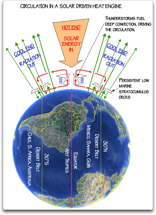
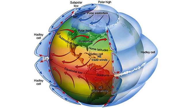
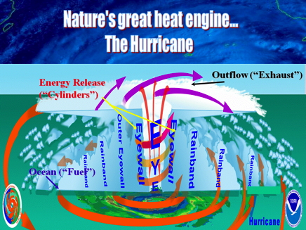
Heat Transport: In order to understand how the heat is transported by the geophysical fluids, one should clarify what sets them into motion. We focus here on the atmosphere. A comprehensive view of the energetics fuelling the general circulation is given by the Lorenz Energy Cycle (LEC) framework. This provides a picture of the various processes responsible for conversion of available potential energy (APE), i.e. the excess of potential energy with respect to a state of thermodynamic equilibrium, into kinetic energy and dissipative heating. Under stationary conditions, the dissipative heating exactly equals the mechanical work performed by the atmosphere. In other words, the LEC formulation allows to constrain the atmosphere to the first law of thermodynamics, and the system as a whole can be seen as a pure thermodynamic heat engine under dissipative non-equilibrium conditions.
Water: On one hand the energy budget is relevantly affected by semi-empirical formulations of the water vapor spectrum, on the other hand the energy budget influences the moisture budget by means of uncertainties in aerosol-cloud interactions and mechanisms of tropical deep convection. A global scale evaluation of the hydrological cycle, both from a moisture and energetic perspective, is thus considered an integral part of an overall diagnostics for the thermodynamics of climate system.
Entropy: From a macroscopic point of view, one usually refers to “material entropy production” as the entropy produced by the geophysical fluids in the climate system, which are not related to the properties of the radiative fields, but rather to the irreversible processes related to the motion of these fluids. Mainly, this has to do with phase changes and water vapor diffusion. Lucarini (2009) underlined the link between entropy production and efficiency of the climate engine, which were then used to understand climatic tipping points, and, in particular, the snowball/warm Earth critical transition, to define a wider class of climate response metrics, and to study planetary circulation regimes. A constraint has also been proposed to the entropy production of the atmospheric heat engine, given by the emerging importance of non-viscous processes in a warming climate.
The goal here is to look at models through the lens of their dynamics and thermodynamics, in the view of enunciated above ideas about complex non-equilibrium systems. The metrics that we here propose are based on the analysis of the energy and water budgets and transports, of the energy transformations, and of the entropy production.

Previous Post: Climate Thinking Out of the Box
It seems that climate modelers are dealing with a quandary: How can we improve on the unsatisfactory results from climate modeling?
Shall we:
A.Continue tweaking models using classical maths though they depend on climate being in quasi-equilibrium; or,
B.Start over from scratch applying non-equilibrium maths to the turbulent climate, though this branch of math is immature with limited expertise.
In other words, we are confident in classical maths, but does climate have features that disqualify it from their application? We are confident that non-equilibrium maths were developed for systems such as the climate, but are these maths robust enough to deal with such a complex reality?
It appears that some modelers are coming to grips with the turbulent quality of climate due to convection dominating heat transfer in the lower troposphere. Heretofore, models put in a parameter for energy loss through convection, and proceeded to model the system as a purely radiative dissipative system. Recently, it seems that some modelers are striking out in a new, possibly more fruitful direction. Herbert et al 2013 is one example exploring the paradigm of non-equilibrium steady states (NESS). Such attempts are open to criticism from a classical position, but may lead to a breakthrough for climate modeling.
That is my layman’s POV. Here is the issue stated by practitioners, more elegantly with bigger words:
“In particular, it is not obvious, as of today, whether it is more efficient to approach the problem of constructing a theory of climate dynamics starting from the framework of hamiltonian mechanics and quasi-equilibrium statistical mechanics or taking the point of view of dissipative chaotic dynamical systems, and of non-equilibrium statistical mechanics, and even the authors of this review disagree. The former approach can rely on much more powerful mathematical tools, while the latter is more realistic and epistemologically more correct, because, obviously, the climate is, indeed, a non-equilibrium system.”
Lucarini et al 2014
Here’s how Herbert et al address the issue of a turbulent, non-equilibrium atmosphere. Their results show that convection rules in the lower troposphere and direct warming from CO2 is quite modest, much less than current models project.
“Like any fluid heated from below, the atmosphere is subject to vertical instability which triggers convection. Convection occurs on small time and space scales, which makes it a challenging feature to include in climate models. Usually sub-grid parameterizations are required. Here, we develop an alternative view based on a global thermodynamic variational principle. We compute convective flux profiles and temperature profiles at steady-state in an implicit way, by maximizing the associated entropy production rate. Two settings are examined, corresponding respectively to the idealized case of a gray atmosphere, and a realistic case based on a Net Exchange Formulation radiative scheme. In the second case, we are also able to discuss the effect of variations of the atmospheric composition, like a doubling of the carbon dioxide concentration.
The response of the surface temperature to the variation of the carbon dioxide concentration — usually called climate sensitivity — ranges from 0.24 K (for the sub-arctic winter profile) to 0.66 K (for the tropical profile), as shown in table 3. To compare these values with the literature, we need to be careful about the feedbacks included in the model we wish to compare to. Indeed, if the overall climate sensitivity is still a subject of debate, this is mainly due to poorly understood feedbacks, like the cloud feedback (Stephens 2005), which are not accounted for in the present study.”
Abstract from:
Vertical Temperature Profiles at Maximum Entropy Production with a Net Exchange Radiative Formulation
Herbert et al 2013
In this modeling paradigm, we have to move from a linear radiative Energy Budget to a dynamic steady state Entropy Budget. As Ozawa et al explains, this is a shift from current modeling practices, but is based on concepts going back to Carnot.
“Entropy of a system is defined as a summation of “heat supplied” divided by its “temperature” [Clausius, 1865].. Heat can be supplied by conduction, by convection, or by radiation. The entropy of the system will increase by equation (1) no matter which way we may choose. When we extract the heat from the system, the entropy of the system will decrease by the same amount. Thus the entropy of a diabatic system, which exchanges heat with its surrounding system, can either increase or decrease, depending on the direction of the heat exchange. This is not a violation of the second law of thermodynamics since the entropy increase in the surrounding system is larger.

Carnot regarded the Earth as a sort of heat engine, in which a fluid like the atmosphere acts as working substance transporting heat from hot to cold places, thereby producing the kinetic energy of the fluid itself. His general conclusion about heat engines is that there is a certain limit for the conversion rate of the heat energy into the kinetic energy and that this limit is inevitable for any natural systems including, among others, the Earth’s atmosphere.
Thus there is a flow of energy from the hot Sun to cold space through the Earth. In the Earth’s system the energy is transported from the warm equatorial region to the cool polar regions by the atmosphere and oceans. Then, according to Carnot, a part of the heat energy is converted into the potential energy which is the source of the kinetic energy of the atmosphere and oceans.
Thus it is likely that the global climate system is regulated at a state with a maximum rate of entropy production by the turbulent heat transport, regardless of the entropy production by the absorption of solar radiation This result is also consistent with a conjecture that entropy of a whole system connected through a nonlinear system will increase along a path of evolution, with a maximum rate of entropy production among a manifold of possible paths [Sawada, 1981]. We shall resolve this radiation problem in this paper by providing a complete view of dissipation processes in the climate system in the framework of an entropy budget for the globe.
The hypothesis of the maximum entropy production (MEP) thus far seems to have been dismissed by some as coincidence. The fact that the Earths climate system transports heat to the same extent as a system in a MEP state does not prove that the Earths climate system is necessarily seeking such a state. However, the coincidence argument has become harder to sustain now that Lorenz et al. [2001] have shown that the same condition can reproduce the observed distributions of temperatures and meridional heat fluxes in the atmospheres of Mars and Titan, two celestial bodies with atmospheric conditions and radiative settings very different from those of the Earth.”
THE SECOND LAW OF THERMODYNAMICS AND THE GLOBAL CLIMATE SYSTEM: A REVIEW OF THE MAXIMUM ENTROPY PRODUCTION PRINCIPLE
Hisashi Ozawa et al 2003

Young Mr Dyson in “Turing’s Cathedral” quotes John Von Neumann as concluding that climate modeling was an inherently fruitless waste of mathematics. The disconnect between raw data graphs at realclimatescience.com and current prophesies by Millerite alarmists confirms this conclusion. Data-tampering is no more a solution than Orwellian “rectifying” of old newspapers in an effort to prop up appearances for predatory socialism. Truth, however, is not popular enough to catch on anytime soon, given the popularity of Faith.
LikeLike
Climate modeling, where only global surface mean temperature is concerned is a ten minute exercise a talented high school.student could perform.
Variants of these simple energy balance models with a Chaney sensitivity of 3C are remarkably accurate. I run sims under various net forcing scenarios using a pair of models(GISS Model 2 and CESM2).
Even the old GISS 2 has proven remarkably accurate to this point.
I am not a climate scientist, but a computational modeler of all manner of complex data. In my 30 years of field work I have been made privy to lots of advancements in climate models.
Without getting technical it is lack of computing power that limits today’s models. I can run the GISS 2 on a single machine with 16 compute cores, while the CESM2 takes days to run a sim on a 128 core Linux cluster.
Even discounting Hamiltonian advances–and it’s still unclear whether non-classical mechanics will achieve more robust results–every increase in either parameter or spatio-resolution requires 10000x the computing power.
Since your blog post the models haven’t changed much. There are a couple of brand new models that were introduced over the summer of 2019, but it remains to be seen if these new models resolve detail better than current models.
The takeaway isn’t how badly even models made in the 1970s have performed, but how well. An analysis of models to observation regarding mean GST was done by Z. Hausfather, and some models overlay the observed GST to the point where it is obvious that the models have high levels of skill without accounting for small scale events.
The uncertainty over cloud decks remains, but even with the uncertainty, the models are highly useful.
I have a few equations regarding cloud formation(simple microphysics of thermal properties and surface genesis) but these are crude tools. I have talked to cloud physics experts and a full accounting of the processes involved is lacking.
If one is concerned with resolving one aspect of future climate regimes, it is best to resolve GST. From there latitudinal variations are well represented. Fine resolution of the hydrological cycle would be next in importance.
In the mid to latter parts of this century, under a business as usual emissions scenario, parts of the earth are likely to become uninhabitable due to excessive heat and aridification. Then it is sea-level rise.
The above scenarios are already playing out. They are also accelerating. Climate refugees are going to be the largest socio-economic stressor later this century.
I noted above that I am not a climate scientist. I have the requisite background in mathematics (MSc Applied Mathematics) and a physics MSc, but I am only smart enough to replicate the work of smarter people.
Beware of outliers in climate science. Many of them have been spectacularly wrong, and the balance simply commonly wrong.
Lots of people use the CESM2 as it’s free and only requires a decent university’s compute power. If you’re really interested in what the model uses for inputs there is wiki here: https://github.com/ESMCI/cime/wiki/CIME-Users-Guide or better find a Uni. near you and ask a few questions. It is a real eye-opener.
LikeLike