Arctic Freezing Week

atl066to074.gif

After stalling first week of March, Arctic ice is coming on strong now.  The image above shows the last week, setting new maximums for 2018 for NH overall, as well in Barents Sea.  The graph below shows that as of yesterday, Barents is well above the 11 year average, and even ahead of 2014 the highest year in the decade.

Barents day074

Meanwhile ice extent is increasing on the Pacific side as well.  Bering rapidly grew 200k km2 in a week, setting a new 2018 maximum, while Okhotsk added 110k km2 for a new max ice extent there.

pac066to074

The graph below shows how strongly the Arctic is now freezing over.

NHday074

Note the average max on day 62 and 2018 max yesterday on day 74, now matching 2007 and 120k km2 above last year.  SII (NOAA) continues to show ~200k km2 less extent.

Drift ice in Okhotsk Sea at sunrise.

The graph below shows 2018 NH ice extents since day 1, with and without the Pacific basins Bering and Okhotsk, compared to 11 year averages (2007 to 2017 inclusive).
NHwBandO074
The deficit is almost entirely due to Bering, with the shortfall closing in the last week.

Bering Ice Deficit Gone in Five Days

An update to yesterdays post  Premature Arctic Ice Fears which discussed lop-sided media coverage of  a temporary ice shortfall in Bering Sea.  Now today, the image above shows that in just five days, that deficit has been obliterated.  Since day 66, Bering added 170k km2 to go over 400k km2, close to the previous Bering high in 2018 on day 34.  That was the last Arctic region where some alarm could be raised.  Overall, 2018 is now higher than 2017 at this date, having reached a new maximum of 14.6M km2.

Premature Arctic Ice Fears

Barents60to70

Click on image to enlarge.

The alarms are sounding about lack of ice extent in Bering Sea, studiously ignoring what else is happening in the Arctic.  For instance the above image shows the last 10 days on the European side, with Barents Sea on the right growing steadily to a new maximum. On the left, Gulf of St. Lawrence ice is retreating as usual while Baffin Bay holds steady.

The Barents recovery is interesting and bears watching.  See how 2018 compares with other years in the Graph below.

Barents day070

Note the recent 2018 dramatic rise above average.  Meanwhile on the Pacific side the seesaw between Bering and Okhotsk continues:
BandO60to70

In the last ten days, Bering has gone up, then down, and back up to arrive at the same extent.  In the same period Okhotsk added 70k km2.

Ice extents for February and March appear in the graph below; 11 year average is 2007 to 2017 inclusive.

Note that ice growth slows down in February and March since the Arctic core is frozen and extent can only be added at the margins.  MASIE shows 2018 is now matching 2017, while SII is running about 200k km2 lower.  The 11 year average maxed on day 62 at 15.1M km2 while this year  max was on day 69, ~560k km2 lower . It remains to be seen what max will end up in 2018

It is natural for alarmists to focus on Bering Sea, since that is the only place where a sizable deficit appears (for the moment).  The graph below show NH ice extent from day 1, with and without B and O (Bering and Okhotsk, the Pacific basins that will melt out by September anyway.)


Here’s your Valentine’s Day Greeting:

And here’s your PC candy for Valentine’s Day.


Bering Sea Reduces Arctic Maximum

Bering035to047

Last month came breathless headlines from Inside Climate News:  Alaska’s Bering Sea Lost a Third of Its Ice in Just 8 Days

The good news was that the ice was found just next door in Okhotsk Sea.  As the image above showed, Bering did reduce its coverage, but Okhotsk was gaining at the same time. Over those 12 days, Bearing lost 173k km2 of ice extent while Okhotsk gained 185k km2.

Now we have perhaps already passed the annual maximum, which on average was 15.1M km2 on day 62.

NH arctic ice day 066r

2018 has reduced ice extent the last three days since peaking on day 63.  It came near to 2007 and 2016 before retreating.  And as in the past, SII is tracking about 200k km2 lower.  The regional extents are shown in the table below.

Region 2018066 Day 066 
Average
2018-Ave. 2017066 2018-2017
 (0) Northern_Hemisphere 14380231 15084354 -704123 14706492 -326261
 (1) Beaufort_Sea 1070445 1070178 267 1070445 0
 (2) Chukchi_Sea 965161 966001 -840 966006 -845
 (3) East_Siberian_Sea 1087120 1087134 -14 1087137 -18
 (4) Laptev_Sea 897845 897842 3 897845 0
 (5) Kara_Sea 934934 926489 8445 912664 22270
 (6) Barents_Sea 624841 647307 -22466 597521 27320
 (7) Greenland_Sea 537737 641220 -103484 615726 -77989
 (8) Baffin_Bay_Gulf_of_St._Lawrence 1557754 1560371 -2617 1545548 12206
 (9) Canadian_Archipelago 853109 852753 356 853214 -106
 (10) Hudson_Bay 1260838 1259900 938 1260903 -66
 (11) Central_Arctic 3152831 3219866 -67035 3223471 -70640
 (12) Bering_Sea 232461 757199 -524738 628542 -396081
 (13) Baltic_Sea 138089 94664 43425 69380 68708
 (14) Sea_of_Okhotsk 1041074 1070088 -29014 953551 87522

The 2018 deficit to average is almost entirely due to Bering Sea lack of refreezing, now 525k km2 below recent normal.  On the European side, Barents and Kara are nearly average, with Greenland Sea down about 20%.  It remains to be seen if this year’s maximum is past or if more extent is gained in the coming week.

Drift ice in Okhotsk Sea at sunrise.

The graph below shows 2018 NH ice extents since day 1, with and without the Pacific basins Bering and Okhotsk, compared to 11 year averages (2007 to 2017 inclusive).  Clearly 2018 is an average year except for the Pacific basins, especially Bering Sea.

Arctic Ice Swirls End of Feb.

Click on image to enlarge.

Under the influence of a split vortex in February, Arctic ice is also a bit bi-polar.  Above image shows the Atlantic side the last two weeks.  Barents on the right has grown back to reach the 11 year average, while on the upper left Baffin Bay is above average reaching down to Newfoundland and filling in the Gulf of St. Lawrence.

Click on image to enlarge.

Meanwhile, the ridge of high pressure over Alaska resulted in Bering on the right losing ice while Okhotsk on the left gained up to last year’s maximum.

Ice extents for February appear in the graph below; 11 year average is 2007 to 2017 inclusive.
Note that ice growth slows down in February since the Arctic core is frozen and extent can only be added at the margins.  MASIE shows 2018 is drawing close to 2007 and 2017, while SII is running about 200k km2 less.  The 11 year average reached 15M km2 while this year is ~500k km2 lower at day 57.

Below is the analysis of regions on day 057.  Average is for 2007 to 2017 inclusive.

Region 2018057 Day 057 
Average
2018-Ave. 2017057 2018-2017
 (0) Northern_Hemisphere 14471633 14982823 -511189 14624988 -153354
 (1) Beaufort_Sea 1070445 1070178 267 1070445 0
 (2) Chukchi_Sea 962774 965725 -2951 966006 -3232
 (3) East_Siberian_Sea 1087120 1087134 -14 1087137 -18
 (4) Laptev_Sea 897845 897842 3 897845 0
 (5) Kara_Sea 928561 922491 6070 933003 -4442
 (6) Barents_Sea 599940 618000 -18061 535489 64451
 (7) Greenland_Sea 405456 639713 -234257 621708 -216252
 (8) Baffin_Bay_Gulf_of_St._Lawrence 1823426 1492225 331201 1490888 332538
 (9) Canadian_Archipelago 853109 852670 439 853214 -106
 (10) Hudson_Bay 1260838 1260663 175 1260903 -66
 (11) Central_Arctic 3076082 3222907 -146825 3217927 -141845
 (12) Bering_Sea 283579 737222 -453642 577660 -294081
 (13) Baltic_Sea 130666 116020 14646 64843 65822
 (14) Sea_of_Okhotsk 1063381 1049659 13722 991862 71519

The 2018 deficit to average is almost entirely due to the shortfall in Bering Sea.  Barents, Chukchi and Okhotsk are all about average.  A large surplus in Baffin Bay/Gulf of St. Lawrence offsets smaller deficits in Central Arctic and Greenland Sea.

The annual maximum usually occurs mid March.  2018 is now 2% below last year’s max and needs 3.5% more extent to reach 15M km2.

Here’s your Valentine’s Day Greeting:

And here’s your PC candy for Valentine’s Day.


Volatile Vortex


Dr. Judah Cohen covers the latest vortex shaninigans and implications for future weather at his always informative website Arctic Oscillation and Polar Vortex Analysis and Forecasts February 19, 2018. Excerpts below with my bolds.  Video above of nullschool wind patterns from October 2017 up to yesterday, showing the vortex splitting as described below.

The stratospheric PV remains split into two pieces with one dominant center over Western Canada and a second much weaker center over northwestern Europe (Figure 12). The Eurasian center is predicted to retrograde westward and dissipate while the North American center slowly drifts north towards the North Pole and even possibly into Eurasia. The most persistent legacy of the PV spit is above normal geopotential heights and warm temperatures in the polar stratosphere. This is reflected in the stratospheric AO, which is predicted to remain negative over the next two weeks, though slowly trend back to neutral (Figure 1).

As I have discussed in previous blogs there seems to me to be two responses to a significant PV disruption: an immediate response and a longer term response. When the PV split it created two sister vortices a dominant center over North America and a more minor center over Eurasia. In between the two PV centers high pressure filled the void but was shifted towards the Eurasian continent. Across Eurasia the immediate and longer term response seem to be consistent. The immediate tropospheric response or at least the tropospheric circulation related to the PV split has been high pressure/heights to the north, low pressure/heights to the south, predominant anomalous easterly flow and below normal temperatures across northern Eurasia.

Figure 2. Observed 500 mb geopotential heights (dam; contours) and geopotential height anomalies (m; shading) for 00Z 19 February 2018.

In contrast the immediate and longer term response across North America do not seem to be the same. When the PV split into two pieces the dominant sister center formed over Western Canada and has been spinning in place in the polar stratosphere. It appears to me this has contributed or at least is related to troughing/negative geopotential height anomalies across Canada and then eventually into the Western US accompanied by colder temperatures. This in turn has forced further downstream across eastern North America ridging/positive geopotential height anomalies, southwesterly flow and mild even record warm temperatures.

Eventually however the Eurasian PV sister center is predicted to weaken and dissipate leaving just one PV center over Western Canada. That PV center is predicted to make its way back to the North Pole or alternatively there are some model forecasts of the PV center being further displaced towards Eurasia.

Longer term the tropospheric response seems to be less about the initial displacement and the associated circulation around the respective PV centers and more about the warming and high pressure/heights related to that warming. The corresponding tropospheric response is high pressure and relatively warm temperatures over the Arctic. With respect to the ongoing event the high pressure and warm temperatures in the polar stratosphere are centered over Greenland and therefore it seems likewise in the troposphere the high pressure/heights and warm temperatures will be centered over Greenland. This transfer of high pressure/heights and warm temperatures over the Arctic is seen in the apparent downward propagation of positive/warm polar cap geopotential heights and/or a negative AO from the mid-stratosphere eventually down to the surface. On average this downward propagation or transfer takes about two weeks.

Figure 5. (a) Forecasted average 500 mb geopotental heights (dam; contours) and geopotential height anomalies (m; shading) across the Northern Hemisphere from 25 February – 1 March 2018. (b) Same as (a) except averaged from 2 – 6 March 2018. The forecasts are from the 19 February 2018 00z GFS ensemble.

Therefore in summary based on my reasoning, the immediate response to a PV disruption is somewhat random dependent on the displacement of the PV center(s) and the circulation around the PV center(s). For the current event the immediate tropospheric response related to the location and circulation of the North American sister vortex favors relatively cold temperatures in western North America and mild temperatures in eastern North America. However the tropospheric response could have just as likely been the opposite favoring relatively mild temperatures in western North America and cold temperatures in eastern North America. Across Eurasia the immediate response favors relatively cold across northern Eurasia and mild temperatures across southern Eurasia; though it does seem that the immediate response across Eurasia is less random than for North America for reasons that I don’t fully understand.

The longer term response or legacy however to a PV disruption is less random and is not as dependent on the location and circulation of the PV center(s) but rather on the warming and building of high pressure/heights across the Arctic which shows greater similarity across PV disruption events. High pressure/heights and warm temperatures favor colder temperatures in preferential locations: the Eastern US, Northern Europe and East Asia resulting in a warm Arctic/cold continents pattern. Therefore my expectations of the longer term response to the ongoing PV disruption is the same – a preference for relatively cold temperatures in the Eastern US, Northern Europe and East Asia over the coming four to six weeks starting the very end of February or the beginning of March.

Forecast for the next month from Environment Canada.


Bering Sea Ice Lost (& Found Next Door)

Bering035to047

Breathless headlines from Inside Climate News:  Alaska’s Bering Sea Lost a Third of Its Ice in Just 8 Days

Well, I have good news for them.  The ice was found just next door in Okhotsk Sea.  As the image above shows, Bering did reduce its coverage, but Okhotsk was gaining at the same time. Over the last 12 days, Bearing lost 173k km2 of ice extent while Okhotsk gained 185k km2. Bering is currently at 35% of last year’s max, while Okhotsk is at 88%, with a month of the freezing season yet to go.

Drift ice in Okhotsk Sea at sunrise.

The graph below shows 2018 NH ice extents since day 1, with and without the Pacific basins Bering and Okhotsk, compared to 11 year averages (2007 to 2017 inclusive).
The deficit comes mostly from Bering Sea, while Okhotsk is above average, and Barents has grown recently.  Greenland Sea and Central Arctic are down to a lesser extent, nearly offset by Baffin surpluses. A month remains to reach annual maximum with the standard this decade being about 15M km2. For perspective, 2018 has to gain about 6% by mid March to reach 15M and gain 4% to reach 14.78, last year’s maximum. It should also be remembered that all of these dancing basins will likely melt out by September as usual.

For a more comprehensive report see Feb. Arctic Ice Dance

Feb. Arctic Ice Dance

For much of February, NH has been overall slower than usual to add ice extent. But that does not mean nothing is happening.  For we can observe ice dances on opposite sides of the Arctic from January up to now. The image above shows how Pacific ice extents have shuffled back and forth between Okhotsk (left) and Bering (right), alternating waxing and waning so that both basins combined are below average. Lately Okhotsk has added ice to reach normal, so now Bering makes most of the difference. Bering is now only 45% of last years maximum, while Okhotsk has reached 81% of last year’s max extent.

Drift ice in Okhotsk Sea at sunrise.

On the Atlantic side, the two players are Barents and Baffin Bay/Gulf of St. Lawrence. On the left side  you can see Baffin Bay extending down to reach Newfoundland, and Gulf of St. Lawrence filling in.  Meanwhile Barents has waffled up and down, first growing to reach Svalbard and then receding along with Greenland Sea opening to the left of Svalbard.  Barents is presently at 75% of last years maximum, while BB/GSL extent is its highest this year and 96% of last year’s max.

Sea ice forming in Baffin Bay.

Overall 2018 Arctic ice has reached 14.1M km2, about 600k km2 or 5% below average.

MASIE shows this year catching up to 2017 while SII 2018 lags ~300k km2 behind.  The graph below shows 2018 NH ice extents since day 1, with and without the Pacific basins Bering and Okhotsk, compared to 11 year averages (2007 to 2017 inclusive).
Clearly the deficit to average is mostly due to B&O, and as the table below shows, mostly Bering at this point.

Region 2018044 Day 044 
Average
2018-Ave. 2017044 2018-2017
 (0) Northern_Hemisphere 14140166 14756619 -616453 14287848 -147682
 (1) Beaufort_Sea 1070445 1070178 267 1070445 0
 (2) Chukchi_Sea 965971 965614 357 966006 -35
 (3) East_Siberian_Sea 1087120 1087134 -14 1087137 -18
 (4) Laptev_Sea 897845 897842 3 897845 0
 (5) Kara_Sea 874714 906136 -31422 908380 -33666
 (6) Barents_Sea 465024 567976 -102952 363927 101097
 (7) Greenland_Sea 529094 630790 -101696 565090 -35996
 (8) Baffin_Bay_Gulf_of_St._Lawrence 1655681 1483847 171834 1564353 91328
 (9) Canadian_Archipelago 853109 853029 80 853214 -106
 (10) Hudson_Bay 1260838 1260792 46 1260903 -66
 (11) Central_Arctic 3117143 3218063 -100920 3209792 -92649
 (12) Bering_Sea 319927 730017 -410090 564241 -244314
 (13) Baltic_Sea 76404 105038 -28634 59994 16410
 (14) Sea_of_Okhotsk 911105 906055 5050 834828 76277

The large deficit comes from Bering Sea, while Okhotsk is matching average, and Barents has grown recently.  Greenland Sea and Central Arctic are down to a lesser extent, nearly offset by Baffin surpluses. A month remains to reach annual maximum with the standard this decade being about 15M km2. For perspective, 2018 has to gain about 6% by mid March to reach 15M and gain 4% to reach 14.78, last year’s maximum. It should also be remembered that all of these dancing basins will likely melt out by September as usual.

Arctic Ice Watch January 31

Click on image to enlarge.

Arctic ice is growing extents slowly to approach 14M km2 with about six weeks left to reach annual maximum.  The meandering polar vortex brings warmer air north to replace the cold air sent into Canada and USA.

The image above shows Barents on the right is finally adding extent, growing 200k km2 in two weeks to reach 76% of last year’s maximum. The image below shows the ice see-saw in the Pacific.  First Okhotsk grows 100k km2 to reach average (63% of maximum) while Bering dithers.  Then Bering adds 100k km2 to reach 53% of maximum (still below average), while Okhotsk retreats, giving back its 100k.

Click on image to enlarge.

Ice extents for January appear in the graph below; 11 year average is 2007 to 2017 inclusive.

Note that 2007 caught and exceeded the 11 year average ending the month tied.  2018 is now ~300k km2 below 2017 and both lag behind average having started the year in deficit. SII 2018 is running about 200k km2 less than MASIE for the month.

Below is the analysis of regions on day 031.  Average is for 2007 to 2017 inclusive.

Region 2018031 Day 031 
Average
2018-Ave. 2017031 2018-2017
 (0) Northern_Hemisphere 13792271 14504082 -711811 14086396 -294125
 (1) Beaufort_Sea 1070445 1070210 235 1070445 0
 (2) Chukchi_Sea 965971 965960 11 966006 -35
 (3) East_Siberian_Sea 1087120 1087023 97 1087137 -18
 (4) Laptev_Sea 897845 897820 24 897845 0
 (5) Kara_Sea 895363 915975 -20612 862890 32473
 (6) Barents_Sea 481947 578898 -96950 421776 60171
 (7) Greenland_Sea 501411 622550 -121139 549359 -47948
 (8) Baffin_Bay_Gulf_of_St._Lawrence 1406903 1362611 44292 1299268 107634
 (9) Canadian_Archipelago 853109 853066 43 853214 -106
 (10) Hudson_Bay 1260838 1260818 19 1260903 -66
 (11) Central_Arctic 3184817 3219924 -35107 3232583 -47766
 (12) Bering_Sea 382207 685972 -303766 509369 -127162
 (13) Baltic_Sea 41714 76231 -34517 31706 10008
 (14) Sea_of_Okhotsk 704398 836881 -132483 1006706 -302308

The core of the Arctic is frozen solid and for the date 2018 is ~5% below average.  The difference is mainly due to Bering Sea 44% below average, Greenland 20% down, Barents 17% less, and Okhotsk 16% lower. 

Postscript:

Check out the action in Kara Sea near the mouth of the Yenisei River, as a nuclear ice breaker comes within meters of a car expedition on the ice, temperatures at -50C. January 26, 2018


Arctic Wonder

I am excerpting from Dr. Cohen’s latest post because of his refreshing candor sharing his thought processes regarding arctic weather patterns. Arctic Oscillation and Polar Vortex Analysis and Forecasts  January 29, 2018 Dr. Judah Cohen.  (my bolds and images added)

I have really struggled with what to discuss in today’s Impacts section and in the end decided to focus on a feature that gets no respect and to elaborate on last week’s discussion. One big problem has been large model uncertainty and lack of reliable guidance. I think it should be obvious to anyone reading the blog that I am focused on the behavior of the stratospheric polar vortex (SPV) and using variability in that behavior to anticipate large scale climate anomalies across the Northern Hemisphere (NH) on the timescale of days to weeks and even months.

The weather models (I spend most of my time analyzing the global forecast system (GFS) but I do not think that it is limited to the GFS) have been predicting some wild and highly anomalous behavior in the SPV. First the GFS was predicting a SPV displacement into North America (why this is highly anomalous is a good question and not something that I fully understand). Then the GFS predicted a strong warming in the polar stratosphere centered over Scandinavia of the magnitude that is only observed over East Asia and Alaska. The GFS has mostly backed off of these forecasts or at least predicting events of much smaller magnitudes (though it is back in the 12z run).

And looking back at the behavior of the SPV for the winter it can be summed up as unremarkable in many ways. My sense is that the SPV has been stronger than normal for the winter characterized a mostly positive stratospheric AO and cold/below normal PCHS in the stratosphere. Based on that alone one would expect an overwhelmingly mild winter across the NH mid-latitudes. However that would not be an accurate description of the winter.

But in the atmosphere you cannot have low pressure without high pressure. And as we head into the final third or half of winter, I don’t think that one can understand or explain this winter’s temperature variability without focusing on anomalous high pressure in the polar stratosphere. So in the end I have decided to discuss what I like to call the “Rodney Dangerfield” of weather- high pressure because it doesn’t seem to get the respect it deserves certainly compared to low pressure.

My passion for weather began with my love for snow and I couldn’t wait for the next snow opportunity. I grew up in New York City (NYC) where it snows every winter but to get a good snowfall is always challenging and predicted snowfalls more often than not did not materialize because of too much dry air or too much warm air or the storm being too far out to sea…. It became apparent to me having an area of low pressure passing near NYC rarely translated to a snowstorm.

Instead a better predictor of snowfall was the position of high pressure. If Arctic high pressure settled to the north of NYC across Quebec or even Northern New England the likelihood of snowfall greatly increased despite model predicted storm tracks. With high pressure entrenched to the north, good things (as far as snow falling in NYC) happened. So even though meteorologists like to focus on storms and low pressure, in my opinion the key player in whether it would snow or not was the high pressure.

This recognition of the importance of high pressure that began with my passion for weather followed me to my studies. On the regional scale of snowfall in NYC it was the storms that got all the attention and high pressure was neglected (at least that was my impression). Similarly when I began studying winter climate variability on a large scale again my impression was that the focus was on the two semi-permanent large scale low pressures the Icelandic and the Aleutian lows.

There was a third semi-permanent feature that seemed to get scant attention – the Siberian high. When my own research demonstrated a relationship between Eurasian snow cover and winter climate including in the Eastern US to me the obvious link or pathway was the Siberian high. It took many years and many studies to come to the understanding I have today (which remains incomplete) but it is my opinion that the Siberian high is the single most important large scale synoptic feature that influences the variability of the SPV (other climate scientists may disagree with me).

My own empirical observations are that when the Siberian high is shifted to the northwest over the Urals and Scandinavia region, this will inevitably produce increased energy transfer from the troposphere to the stratosphere and more often than not disrupt the SPV. The likelihood of a disruption will increase if the Ural blocking is coupled with downstream troughing across East Asia and the North Pacific or a deeper than normal Aleutian low.

Through the blog I advocate for the importance of SPV variability on sensible weather and whether the SPV is “still” or “disrupted” can have important and large implications for surface weather. As I discussed last week, from the blog it has become obvious to me thinking of the SPV as weak and strong only, or even compositing based on the absence or existence of zonal wind reversals at 60°N and 10 hPa was overly simplistic and probably missed most of the coupling with the troposphere. Instead the position of the SPV and the flow around the SPV were important regardless of the speed of the zonal winds at 60°N and 10 hPa.

But this winter makes me believe that it might even be more nuanced than even the wind flow around the SPV. The precursor to the historic cold in the Eastern US in late December and early January was a Canadian warming/high pressure in the polar stratosphere the third week of December. But as it turns out the most impressive cold anomalies during the month of January are not in North America but Asia. A second warming/high pressure near Eastern Siberia in mid-January accompanied near record cold in Siberia and large parts of Asia.

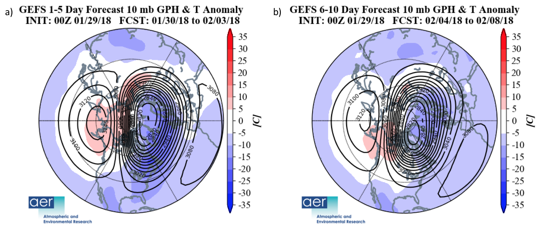
Figure 12. (a) Forecasted 10 mb geopotential heights (dam; contours) and temperature anomalies (°C; shading) across the Northern Hemisphere for 30 January – 3 February 2018. (b) Same as (a) except averaged from 4 – 8 February 2018. The forecasts are from the 29 January 2018 00z GFS ensemble.

Now a third warming/high pressure predicted back in the western hemisphere across Alaska and Northwest Canada is again a precursor for a return of cold temperatures to the Eastern US and Eastern Canada starting this week (see Figure 12). The location of high pressure/heating in the polar stratosphere is the best explanation that I have for the placement and timing of the dominant cold anomalies across the NH. I have a hard time making the same explanation based on the location of the SPV or the flow around the SPV.

Of course my reasoning is overly simplistic and the resultant weather anomalies are not limited to one factor or influence but rather a combination of many different influences or forcings. As I discussed in last week’s blog an alternative explanation being offered for the return of cold weather to eastern North America is the Madden Julian Oscillation (MJO). 

Originally the models and meteorologists relying on MJO forcing predicted a mild first half of February and a colder second half of February. That forecast has changed mostly to a cold February from start to finish. I don’t think that change in the forecast can be ignored or glossed over with the change in timing as an inconsequential detail. The forecast for this week across the US is western ridge and warm with eastern trough and cold, though admittedly the cold is not overly impressive.

Based purely on the MJO the next two weeks should feature a cold Western US and a warm Eastern US opposite of the most recent forecasts. If it is cold in the Eastern US over the next two weeks it is not because of the MJO but in spite of the MJO. Currently the models are not quite sure if the MJO will make it to phase 8 but that phase is related to a warm Western US and cold Eastern US. If the cold persists until the third week of February then the MJO forcing could constructively interfere with the already cold pattern.

If the early arrival of the cold cannot be attributed to MJO forcing then what could be the reason? My explanation is something that I have discussed many times before – the models fail to correctly “propagate down” circulation anomalies from the stratosphere to the troposphere until the changes can’t be ignored. At longer leads the models did not correctly predict the return of Alaska ridging related to SPV variability but corrected at shorter leads.

Thanks Dr. Cohen for illuminating the art and science of studying the weather in its fascinating complexity.  More on his forecasting paradigm at Warm is Cold, and Down is Up