Arctic Sea Ice | Science Matters

Arctic Ice Minimums Compared

Posted on September 20, 2015 by Ron Clutz

Update Sept. 20, 2015: 2014 and 2015 Minimums Established, 11 days ago in NOAA, 2 days ago in MASIE

In the annual match of the ocean vs. Arctic ice, Mother Nature has blown the whistle. Results are little confusing, since NOAA shows the lowest extent 11 days ago, and MASIE only 2 days ago. Moreover, MASIE dropped a lot of ice in the recent period and is now showing less ice than NOAA. Usually, MASIE is higher by 2-300k km2.

Still, for the climate record it will be the September average that counts, and the platform is firmed up for that result.

First the daily situation:

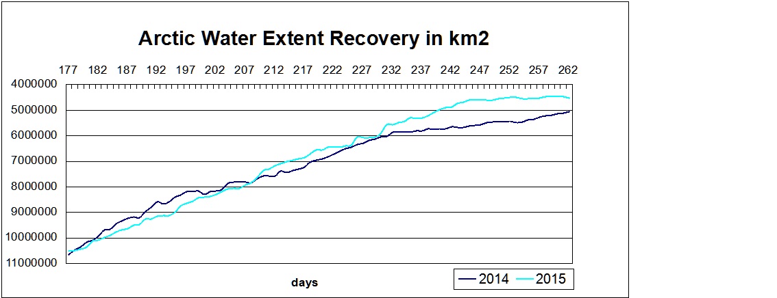
September 19 day 262 results from MASIE. 2014 loses a lot while 2015 gains a lot of ice extent.

While 2014 lost 46k of ice, 2015 gained 70k recovering well above the previous annual daily ice minimum..

2015 ice extent now trails 2014 by 10.6%, which is about 538k km2 difference. Day 262 is the 2014 daily ice extent minimum. Day 260 was 2015 minimum, according to MASIE.

Comparing 2014 and 2015 at Annual Minimums

Ice Extents	Day 2014262	Day 2015260	Ice Extent
Region	Ann Min	Ann Min	km2 Diff.
(0) Northern_Hemisphere	5066134	4442258	-623876
(1) Beaufort_Sea	655536	484880	-170656
(2) Chukchi_Sea	235122	187420	-47701
(3) East_Siberian_Sea	455832	219274	-236559
(4) Laptev_Sea	1212	44701	43489
(5) Kara_Sea	64255	1778	-62478
(6) Barents_Sea	132741	18	-132723
(7) Greenland_Sea	210190	236707	26517
(8) Baffin_Bay_Gulf_of_St._Lawrence	18245	57136	38891
(9) Canadian_Archipelago	341623	228074	-113549
(10) Hudson_Bay	862	47674	46811
(11) Central_Arctic	2949375	2933456	-15919

The table shows the effects of weather in the western Arctic. In August 2015 lost 700k km2 more than 2014, a differential that persisted to the minimum. The reductions occurred in the BCE region and in the near by CAA (Canadian Archipelago). In addition in the east, Barents melted out early and entirely, and nearby Kara become mostly open water.

Elsewhere, on the Canadian side, Hudson and Baffin Bay along with the Greenland Sea had more ice, and the Central Arctic was nearly the same as in 2014.

2015 Recap:

The first 19 days of September 2015 is in the books, so here is an outlook on the melt season conclusion beyond the daily minimums.

For most of the season, 2015 Arctic sea ice extent was tracking 2014. In fact the July average extent was slightly higher than 2014. Then weather intervened in the last week of August. A large and strong cyclone centered over Chukchi Sea began breaking up ice in the BCE Region and affecting CAA (Canadian Archipelago) and the Central Arctic. In addition, most of the summer the Arctic Oscillation (AO) was in negative phase, meaning fewer clouds, more direct insolation and ice melting. More discussion of these two factors is at the end of this post.

The effects of this storm are seen in the rapid increase in water extent ( 482k km2 in one week) so that August 31 2015 had less ice than did 2014 at minimum September 19. Water extent continued to grow, and then stabilized once the storm abated and the AO went from negative to neutral. Now the ice is growing beyond the daily minimum.

Comparing MASIE and NOAA Ice Extents.

Month	2015	2015	2015	2014	2014	2014
Ave.	MASIE	NOAA	MASIE-NOAA	MASIE	NOAA	MASIE-NOAA
Feb				15.032	14.498	0.534
March				15.170	14.758	0.413
April	13.650	13.954	-0.304	14.318	14.088	0.230
May	12.646	12.485	0.161	12.916	12.701	0.215
June	10.841	10.889	-0.049	11.324	11.033	0.292
July	8.713	8.411	0.302	8.482	8.108	0.374
August	5.961	5.658	0.303	6.353	6.078	0.275
Sept	4.545	4.463	0.082	5.364	5.220	0.144
Oct				7.697	7.232	0.464

The table shows July 2015 was above 2014 but late August weather caused a drop in monthly averages. The August average is now complete and shows ice extent dropped ~2.7M km2 from July, compared to a 2014 loss of ~2.0M. That difference has persisted up to today. NOAA typically reports a lower extent than MASIE, a difference that averaged ~300k km2. Then in one week MASIE dropped while NOAA plateaued, and now NOAA September extents are quite close to MASIE, some days showing a higher number.

With the September daily ice starting out lower than 2014 the monthly average should end up much smaller. The September first 19 days average is shown, a figure that should rise and end the month near 4.6M km2. This presumes the minimum has definitely occurred, and the recovery is in effect.

In any case, I am not alarmed over open water in the Arctic. Steadily increasing and above average September ice extents signify the coming of the next ice age, a genuine threat to human life and prosperity. Fortunately, that is not the indication this year.

Current and Recent Weather in the Arctic

In addition to the storm, the negative AO has been conducive to accelerating ice melting by increased insolation.

September 16 Arctic Oscillation Forecast from AER:

The AO, which has remained almost consistently in negative territory since late June, has resulted in near record low AO values for July and August. The AO is predicted to first trend positive through the weekend and pop into positive territory early next week. However by midweek the AO is predicted to return back into negative territory and remain negative through early October.

“The positive trend in the AO and the setting sun may have brought an early end to the Arctic sea ice melt season but not before sea ice extent achieved its fourth lowest value since observations began. It is likely that the extremely low AO values observed in July and August are reflective of atmospheric conditions (sunny and warm) that were conducive to rapid sea ice melt.”

https://www.aer.com/science-research/climate-weather/arctic-oscillation

The Alaska Dispatch News reported August 27 on the storm effects at Barrow, Alaska:

“The service has issued a coastal flood warning for Barrow until Friday morning, along with a high surf advisory for the western part of the North Slope and a gale warning for much of the Beaufort and Chukchi Seas. Seas up to 14 feet were forecast for Thursday in the Chukchi. . .Thursday’s high waves and flooding are products of a large storm that’s being felt as far as Southcentral Alaska, where high winds are forecast, Metzger said. “It’s a pretty big low-pressure system that’s over the Arctic Ocean,” he said. ”

https://www.adn.com/article/20150827/high-winds-causing-big-waves-flooding-barrow

a quarter million square KM of arctic ice in the CAB, adjacent to the Beaufort and Chukchi. 20150829

This storm is reminiscent of the 2012 event that resulted in the lowest ice, greatest water extent this century. The high winds, waves and swells have several effects: Gales push ice floes, opening water between them and pushing them toward warmer waters; Ice pieces are churned and fractured increasing the melt rate; Wave action can flood ice packs or can cause compacting, further reducing extent.

Seeing the Arctic Melt without Warmist Glasses

Posted on August 20, 2015 by Ron Clutz

In my Arctic Ice Watch reports I have been tracking progress toward September minimum with graphs like these (data from MASIE):

Doing this after a 3-week break, I was struck by the chart looking a lot like the scoring summary of a tight basketball game, only upside down.

Then AndyG55 commented on my recent summary by linking to this chart from Ed Hoskins:

As the above diagram shows, the temperature balance was pretty close for 7000 years, until the cooling accelerated over the last 3000 years.

My light bulb was in seeing that the summer melt is actually the enormous effort by the ocean to recover water trapped as sea ice in the Arctic. The ice extent varies greatly over the centuries and we know from artifacts that it has been both greater and smaller than presently. In this time of global warming alarmism, some of us watching the melt season find ourselves hoping for the ice to gain extent, simply to take away that basis for claiming the end is nigh.

Let’s be clear. In this contest between the ice and ocean, we humans should be rooting for the ocean, and so would plants and animals if they knew what was going on. None of us want another ice age, so it is a good thing that the ocean has been gaining on the sea ice extent in the last 150 years.

Once again warmists have got it backwards. The Arctic is a canary all right: The more ice there is in September, the closer we are to the next ice age. Open water in the Arctic is a good thing for the ocean and for the planet.

So taking off the warmist glasses, we should be cheering as the water extent grows and the ice retreats. We don’t wish for a record low because that would drive the alarmists into a frenzy. Anything around 5M km2 for September would signify nothing unusual is happening, so scary things must be found elsewhere.

Maybe the chart should look like this to emphasize the positives of more water, less ice.

Conclusion:
I am not so naive to think that this perspective has much chance against the warmist PR juggernaut. Already the lessening of Antarctic sea ice this year is trumpeted as proof of CO2 warming, and not a celebration of fresh water added to the ocean.

The largest ice cap in the Eurasian Arctic – Austfonna in Svalbard – is 150 miles long with a thousand waterfalls in the summer.

But as Erasmus (1466-1536) said:
In the kingdom of the blind, the one-eyed man is king.

And this one also applies:

Men, it has been well said, think in herds; it will be seen that they go mad in herds, while they only recover their senses slowly, and one by one.
Charles Mackay. Extraordinary Popular Delusions and the Madness of Crowds (1841)

Iceland vs. Greenland, and all that

Posted on August 19, 2015 by Ron Clutz

Why is it that Greenland is mostly ice and Iceland is mostly green?

Many explanations have been offered, usually along the lines of deception: Iceland was so called to discourage others from emigrating, and OTOH Greenland was named to attract others to resettle from Iceland. It seems that after a Viking internal power struggle, the loser and his followers could be banished to leave on a ship to find another land, or die at sea. Thus did Leif Ericsson venture from Iceland to Greenland to found a colony, and later to reach Vinland in today’s Newfoundland.

Leif Ericsson memorial in front of Reykjavik cathedral.

But it may not be deception at all. When you are off the southeastern coast of Iceland, where the Vikings probably approached, and the sun breaks through for a time, you may be treated to this sight:

Iceland Glacier August 5, 2015 sailing southeast of Iceland.

It happens that the Icelandic glacier sits prominently there, and so, it is land alright, but covered with ice. Of course, later on, they discovered the much more liveable western and southern parts and settled there, but maybe the original name stuck.

Meanwhile in Greenland, I was looking for the icecap and was told by our Inuit guide at Paamiut that you have to sail far up the right fjords to see the ice. Even though 90% of Greenland is ice-covered, that is not what you see from the shore.

Near Nuuk Greenland August 31, 2015

Brought to you by:

Follow the Water–Arctic Ocean Flywheels

Posted on July 20, 2015 by Ron Clutz

The motto of oceanography should be: “It’s not that simple.”

Dallas Murphy wrote that in a book containing his reflections from numerous voyages with ocean scientists, entitled Follow the Water: Exploring the Sea to Discover Climate. The author goes on to say:

“One reason why the ocean has been left out of the climate-change discussion is that its internal mechanisms and its interactions with the atmosphere are stunningly complex. That the ocean has been left out has helped pitch the discussion toward unproductive, distracting extremes–either global warming is bunk or sea levels are about to rise twenty feet–and to frame the issue as a matter of opinion, like the place of prayer in public schools.”

He also quotes respected Oceanographer Carl Wunsch: “One of the reasons oceanography has a flavor all it’s own lies in the brute difficulty of observing the Ocean.”

A previous post on the Climate Water Wheel referred to the metaphor of the ocean serving as a thermal flywheel in our planetary climate due to the massive storage of solar energy in bodies of water. Another post provided some basics on the dynamics of sea ice.

Now, in keeping with the motto above, we shall see that indeed, it is not that simple when we look more closely inside the Arctic Ocean. For example, consider this map from Woods Hole Oceanographic Institution (WHOI):

“Follow the water: Cold, relatively fresh water from the Pacific Ocean enters the Arctic Ocean through the Bering Strait. It is swept into the Beaufort Gyre and exits into the North Atlantic Ocean through three gateways (Fram, Davis, and Hudson Straits). Warmer, denser waters from the Atlantic penetrate the Arctic Ocean beneath colder water layers, which lie atop the warmer waters and act as a barrier preventing them from melting sea ice.

Once in the Arctic Ocean basin, the water is swept into a mammoth circular current—driven by strong winds—called the Beaufort Gyre (BG). Mighty Siberian and Canadian rivers also drain into the gyre to create a great reservoir of relatively fresh water. Winds trap this water in a clockwise flow, but periodically, the winds shift and the gyre weakens, allowing large volumes of fresh water to leak out. This is “the flywheel,” said WHOI physical oceanographer Andrey Proshutinksy, and when it turns off, fresh water flows toward the North Atlantic.

The water exits the Arctic Ocean via several “gateways.” It can flow through the Fram Strait, between northeast Greenland and Svalbard Island, and then branch around either side of Iceland. It can flow around the west side of Greenland through Baffin Bay and out Davis Strait. It may also flow through a maze of Canadian islands and out Hudson Strait.
These gateways are two-way: They also let in the warmer Atlantic waters that—if not for the halocline—could melt Arctic sea ice.”

http://www.whoi.edu/oceanus/feature/is-global-warming-changing-the-arctic

The BG Flywheel System

The research indicates that the complexity can be imagined as a series of flywheels, interacting and combining to moderate the short term effects of weather and changes in circulations of water and winds. Note that this conception shows the ocean flywheel as having four components or layers that operate in their own patterns while being interconnected.

And, as the flywheel system depicts, the ocean components are stratified by both temperature and salinity (saltiness). When sea ice forms, it releases salt into surface waters. These waters become denser and sink to form the Arctic halocline, a layer of cold water that acts as barrier between sea ice and deeper warmer water that could melt the ice. (Illustration by Jayne Doucette, WHOI)

Arctic Sea Ice Uncertainties

Posted on July 13, 2015 by Ron Clutz

The largest ice cap in the Eurasian Arctic – Austfonna in Svalbard – is 150 miles long with a thousand waterfalls in the summer.

About NOAA and MASIE Ice Extent Statistics

As we approach the serious Arctic melting season toward the September minimum, it is important to have a context to interpret various upcoming media reports.

Two factors are paramount: 1) The Sea Ice Prediction Network (SIPN) uses the September Monthly Average as reported by NOAA; and 2) This year NOAA adjusted its measurement system, resulting in a difference in extent statistics.

NOAA says this:

March 2015
The Sea Ice Index processing was updated to use the smaller SSMIS pole hole instead of the SMM/I pole hole, and the erroneous use of the SMMR pole hole in SSM/I and SSMIS data was also corrected. In addition, a new residual weather climatology mask was applied to the Northern Hemisphere that better represents where ice will and will not be, and the extent values in the daily extent data files have been rounded to three decimal places instead of six because that is the precision of the data. The entire time series was reprocessed and now reflects these changes.

http://nsidc.org/data/docs/noaa/g02135_seaice_index/#mar-2015

As many are aware, NOAA numbers come entirely from passive microwave sensors on satellites, while MASIE ice charts are prepared by the National Ice Center based on multiple sources, including the microwave results, but also satellite imagery and field reports. More of the difference in methodologies and historical results is described here:
https://rclutz.wordpress.com/2015/03/31/comparing-noaa-and-masie-arctic-ice-extent/

Something Different This Year

At the moment we are seeing that NOAA is now reporting ice extent figures that are much closer to MASIE than previously. The following table shows the comparison.

Monthly	2015	2015	2015	2014	2014	2014
Averages	MASIE	NOAA	MASIE-NOAA	MASIE	NOAA	MASIE-NOAA
February				15.032	14.498	0.534
March				15.170	14.758	0.413
April	13.650	13.954	-0.304	14.318	14.088	0.230
May	12.646	12.485	0.161	12.916	12.701	0.215
June	10.841	10.889	-0.049	11.324	11.033	0.292
July	9.573	9.473	0.100	8.482	8.108	0.374
August				6.353	6.078	0.275
September				5.364	5.220	0.144
October				7.697	7.232	0.464

All figures are in M km2. MASIE results stopped last year after October and did not resume until April 2015. The July 2015 average includes only the first 12 days, so it can not be compared to July 2014 30-day average.

Note that last year MASIE showed higher extents in all months, ranging higher by 200-500k km2, except for the September minimum. However, in 2015 NOAA changes show results much closer to MASIE, at times even larger extents. June was almost the same, something that didn’t happen in the past.

Summary

In some charts showing Arctic daily ice extent from several years, NOAA 2015 results exceed 2014 partly because of an adjusted system. The newer numbers are more in synch with MASIE results.

So far 2015 monthly averages are running slightly below last year when comparing MASIE to itself, or NOAA to itself. And SIPN median prediction is for a slightly lower minimum.

However, in the last 2 weeks 2015 is showing higher extent than the same period last year, presently an increase of ~ 500k km2. Will that trend continue?

What will NOAA show in September? In addition to natural uncertainty, some differences may arise from system changes. At least this time, the adjustments are not in an alarming direction.

NOAA data is here:

ftp://sidads.colorado.edu/DATASETS/NOAA/G02135/north/daily/data/

MASIE Update July 13, 2015

2015 retains 2% lead over 2014 in BCE Region

Some Arctic ice watchers are focused on the BCE region: Beaufort, Chukchi and East Siberian Seas. It seems that when multi-year ice collects in this region, the Arctic Sea ice margin is protected, and the melting is reduced, resulting in a higher September minimum. Thus an early melting in BCE region can signal a lower summer minimum for NH ice extent, and vice-versa.

To monitor this, I have added a BCE index, being the total 2015 ice extent in BCE as a % of total 2014 extent in the same region. All figures from MASIE.

Note that the BCE maximum ice extent is comparable in size to Arctic Sea max. Historically BCE melts much more than the Arctic Sea; for example, in 2014 BCE lost 58% of its max compared to only 10% for Arctic Sea.

BCE Index recent results:

Day	BCE 2015	% of 2014
187	2597170	100.2%
188	2594289	99.8%
189	2593287	99.2%
190	2538316	99.1%
191	2540197	100.6%
192	2534781	102.8%
193	2529403	102.6%

Part of the interest in BCE this year comes from the warm water blob in the N. Pacific, that may add melting to this region located on the Asian side. The two years were virtually identical with little melting prior to day 130. Daily losses since then have been similar and the 2 years were tied on day 146. For 3 days 2015 took some losses while 2014 held on to gains. Since day 150 the gap has been ~3-4%, until recently.

The Blob may have melted out Bering Sea early, and that may now be causing Chukchi to have lower extent than last year. Yet the BCE region had more ice than 2014 for 13 days until slipping behind for 3 days, then recovering to again lead by 2%.

For more on the Blob: https://rclutz.wordpress.com/2015/06/13/how-about-that-blob-june-13-update/

July 13, 2015

Day 193, July 12 results from MASIE. Arctic ice extent lead over 2014 dips to 471k km2: A day when 2014 regains ice while 2015 has a small loss. .

2014 gained 58k on this day while 2015 lost 21k, reaching a new seasonal minimum of 9.13M km2. The loss is now 37.2% from NH max on day 93.

2014 extent now trails 2015 by 5.4%, which is about 471k km2 difference.

2015 losses were spread, the largest being 10k in Chukchi.

The seas that have lost ice are: (% lost from each sea’s max)

Baltic 100%
Bering 100%
Okhotsk 99.2%
Barents 87.8%
Baffin Bay 73.7%
Kara 71.1%
Hudson Bay 49.6%
Chukchi 39.2%
Greenland 27.8%
Laptev 19.2%
Beaufort 13.3%
Can Archipelago 12.4%
East Siberian 6.7%

The other seas have lost less than 5% from their maximums.

The seas contributing most to the total NH ice extent loss:

(5) Kara_Sea 12.0%
(6) Barents_Sea 9.6%
(8) Baffin_Bay_Gulf_of_St._L 23.4%
(10) Hudson_Bay 11.3%
(12) Bering_Sea 12.2%
(14) Sea_of_Okhotsk 11.4%

2015 melt still trails 2014 by 5 days.

Outlook:

At this point, the median outlook for NH ice extent average for September 2015 is about 5M km2, slightly below last year. That seems reasonable to me, given the lower March max, but also considering the higher ice thickness. Of course, there is no predicting what weather events will affect the ice melting and compacting between now and October.

What’s at stake this year? If September average is higher than last year, then it supports the recovery narrative. Slightly lower than 2014 (the consensus prediction) and the generally declining trend is supported. A major fall off in ice extent would be followed by mass media alarm bells.

How About That Blob? (June 13 Update)

Posted on June 13, 2015 by Ron Clutz

June 13, 2015

As hoped for by Paris COP promoters, and by Californians looking for El Nino precipitation, the Blob in the North Pacific has intensified and may at least partly fulfill both expectations.

HADSST3 results for May are now in, and the sea surface temperature warming anomaly is up:

Global +0.12C over last May,
NH +0.16C over last May.

That will show up also in air temperature estimates, since 71% of the earth’s surface is covered by oceans. For example, UAH TLT anomalies show Global oceans +0.06C over last May, but Global land -0.1C, so Global UAH is only up +0.02C over May 2014. (Note: UAH uses satellites to measure air temperatures many meters above land or ocean, while surface datasets like HADCRUT, BEST, GISTEMP use the measured SSTs in their global mean temperature estimates).

The Blob difference shows up in UAH in the NH results: NH anomaly is +0.07 over last year, with the same increase showing over land and ocean. Interestingly, UAH shows the North Pole cooler than a year ago, the TLT over the Arctic being -0.06 less than a year ago. The South Pole land air temps are a whopping -0.2C colder than last May.

As far as Arctic Ice is concerned, the Blob probably caused the Bering Sea to melt out more than one month earlier than last year. About 10% of the water entering the Arctic Ocean comes from Bering, so there should be some impact on ice melting the immediate BCE region (Beaufort, Chukchi, East Siberian Seas). So far, in that region, 2015 is tracking last year’s melt at a slightly lower extent -4%, not yet a significant effect from the Blob.

Spitsbergen Triangle: Ground Zero for Climate Mysteries

Posted on June 8, 2015 by Ron Clutz

Credit to Dr. Bernaerts for his writings on this subject, excerpts of which appear below.

The Island Nexus for Ocean Currents

From the Dutch: spits – pointed, bergen – mountains

The largest and only permanently populated island of the Svalbard archipelago in northern Norway. Constituting the westernmost bulk of the archipelago, it borders the Arctic Ocean, the Norwegian Sea, and the Greenland Sea. Spitsbergen covers an area of 39,044 km2 (15,075 sq mi), making it the largest island in Norway and the 36th-largest in the world.

The fact is that the winter temperatures made a jump of more than eight degrees Celsius at the gate of the Arctic Basin, after 1918. Nowadays, one century later, the event is still regarded as “one of the most puzzling climate anomalies of the 20th century”.

Dr. Bernaerts:

The overriding aspect of the location is the sea; the sea around Spitsbergen, the sea between particularly the Norwegian, the Greenland, and the Barents Seas (Nordic Sea). The Norwegian Sea is a huge, 3000 metres deep basin. This huge water mass stores a great amount of energy, which can transfer warmth into the atmosphere for a long time. In contrast the Barents Sea, in the southeast of Spitsbergen has an average depth of just around 230 metres. In- and outflow are so high that the whole water body is completely renewed in less than 5 years. However, both sea areas are strongly influenced by the water masses coming from the South. The most important element is a separate branch of the North Atlantic Gulf Current, which brings very warm and very salty water into the Norwegian Sea and into the Spitsbergen region. Water temperature and degree of saltiness play a decisive role in the internal dynamics of the sea body. And what might be the role of the huge basin of the Arctic Ocean, 3000 meters depth and a size of about 15 million square kilometers?

The difference towards the other seas mentioned is tremendous. The Arctic Ocean used to be widely ice covered in the first half of the 20th Century, the other seas only partly on a seasonal basis. Only between the open sea and the atmosphere an intensive heat transfer is permanently taking place. Compact sea ice reduces this transfer about 90% and more, broken or floating ice may change the proportion marginally. In this respect an ice covered Arctic Ocean has not an oceanic but ‘continental’ impact on the climate.

The Arctic Ocean is permanently supplied with new water from the Gulf Current, which enters the sea close at the surface near Spitsbergen. This current is called the West Spitsbergen current. The arriving water is relatively warm (6 to 8°C) and salty (35.1 to 35.3%) and has a mean speed of ca. 30 cm/sec-1. The warm Atlantic water represents almost 90% of all water masses the Arctic receives. The other ~10% comes via the Bering Strait or rivers. Due to the fact that the warm Atlantic water reaches usually the edge of the Arctic Ocean at Spitsbergen in open water, the cooling process starts well before entering the Polar Sea.

A further highly significant climate aspect of global dimension is the water masses the Arctic releases back to oceans. Actually, the outflow occurs mainly via the Fram Strait between Northeast Greenland and Spitsbergen, and together with very cold water from the Norwegian Sea basin the deep water spreads below the permanent thermocline into the three oceans.

http://www.arctic-heats-up.com/pdf/chapter_2.pdf

The Spitsbergen Event 1918-1919

Beginning around 1850 the Little Ice Age ended and the climate began warming. Before that, at least since 1650 marked the first climatic minimum after a Medieval warm period, the Little Ice Age brought bitterly cold winters to many parts of the world, most thoroughly documented in the Northern Hemisphere in Europe and North America. The decreased solar activity and the increased volcanic activity are considered as causes. However, the temperature increase was remote and once again effected by the last major volcanic eruption of the Krakatoa in 1883. Up to the 1910s the warming of the world was modest.

Suddenly that changed. In the Arctic the temperatures literally exploded in winter 1918/19. The extraordinary event lasted from 1918 to 1939 is clearly demonstrated in the graph showing the ‘Arctic Annual Mean Temperature Anomalies 1880 – 2004’. But this extraordinary event has a number of facets, which could have been researched and explained. Meanwhile almost a full century has passed, and what do we know about this event today? Very little!

Studies considering the causation of the warming offer sketchy rather than well founded ideas. Here are a few examples:
• Natural variability is the most likely cause (Bengtsson, 2004);
• We theorize that the Arctic warming in the 1920s/1930s was due to natural fluctuations internal to the climate system (Johannessen, 2004).
• The low Arctic temperatures before 1920 had been caused by volcanic aerosol loading and solar radiation, but since 1920 increasing greenhouse gas concentration dominated the temperatures (Overpeck, 1997).
• The earlier warming shows large region-to-region, month-to-month, and year-to-year variability, which suggests that these composite temperature anomalies are due primarily to natural variability in weather systems (Overland, 2004).
• A combination of a global warming signal and fortuitous phasing of intrinsic climate patterns (Overland, 2008).

Arctic Regime Change

These explanations (and others such as CO2 or the AMOC) do not come to grips with how extreme and abrupt was this event. In the Spring of 1917, sea ice reached all the way to Spitsbergen, the only time in a century.

And the next year, temperatures rocketed upward, as shown by the weather station there:

A look at the SST history shows clearly an event as dramatic as a super El Nino causing a regime change. But this is the Atlantic, not the Pacific. Cooling followed, but temperatures stayed at a higher level than before.

Summary

The warming at Spitsbergen is one of the most outstanding climatic events since the volcanic eruption of Krakatoa, in 1883. The dramatic warming at Spitsbergen may hold key aspects for understanding how climate ticks. The following elaboration intends to approach the matter from different angles, but on a straight line of thoughts, namely:

WHERE: the warming was caused and sustained by the northern part of the Nordic Sea in the sea area of West Spitsbergen the pass way of the Spitsbergen Current.
WHEN: The date of the commencement of warming can be established with high precision of few months, and which was definitely in place by January 1919.
WHY: the sudden and significant temperature deviation around the winter of 1918/19 was with considerable probability caused, at least partly, by a devastating naval war which took place around the British Isles, between 1914 and 1918.

There is much more evidence and analysis supporting Dr. Bernaerts’ conclusions here:

http://climate-ocean.com/arctic-book/index.html

Conclusion: Unless your theory of climate change can make sense of the Spitsbergen Event, then it cannot inspire confidence. You may not be entirely convinced by Dr. Bernaerts’ explanation, but he at least has one–nobody else has even tried.

Climate on Ice: Ocean-Ice Dynamics

Posted on May 26, 2015 by Ron Clutz

Update May 30, 2015 Longer term context by E.M. Smith added below

Sea ice is not simple. Some Background is in order.

When white men started to explore the north of America, they first encountered the Crees. Hudson Bay posts were established to trade goods for pelts, especially the beavers used for making those top hats worn by every gentleman of the day.

The Crees told the whites that further on toward the Arctic Circle there were others they called “eskimos”. The Cree word means “eaters of raw meat” and it is derogatory. The Inuit (as they call themselves) were found to have dozens of words for snow, a necessary vocabulary for surviving in the Arctic world.

A recent lexicon of sea ice terminology in Nunavik (Appendix A of the collective work Siku: Knowing our Ice, 2008) comprises no fewer than 93 different words. These include general appellations such as siku, but also terms as specialized as qautsaulittuq, ice that breaks after its strength has been tested with a harpoon; kiviniq, a depression in shore ice caused by the weight of the water that passed over and accumulated on its surface during the tide; or iniruvik, ice that cracked because of tide changes and that the cold weather refroze.

http://www.thecanadianencyclopedia.ca/en/article/inuit-words-for-snow-and-ice/

With such complexity of ice conditions, we must recognize that any general understanding of ocean-ice dynamics will not be descriptive of all micro-scale effects on local or regional circumstances.

Short Term Sea Ice Freezing and Melting Cycle

Alarmists only mention positive feedbacks from ice melting, so one is left to wonder why there is any Arctic ice left so many years since the Little Ice Age ended around 1850. Actually there are both positive and negative feedbacks, with one or the other dominating at different times and places.

Of course, the basic cycle is the seasonality of sunless winters and sunlit summers.

Remember that ice grows because of a transfer of heat from the relatively warm ocean to the cold air above. Also remember that ice insulates the ocean from the atmosphere and inhibits this heat transfer. The amount of insulation depends on the thickness of the ice; thicker ice allows less heat transfer. If the ice becomes thick enough that no heat from the ocean can be conducted through the ice, then ice stops growing. This is called the thermodynamic equilibrium thickness. It may take several years of growth and melt for ice to reach the equilibrium thickness. In the Arctic, the thermodynamic equilibrium thickness of sea ice is approximately 3 meters (9 feet). However, dynamics can yield sea ice thicknesses of 10 meters (30 feet) or more. Equilibrium thickness of sea ice is much lower in Antarctica, typically ranging from 1 to 2 meters (3 to 6 feet).

Snow has an even higher albedo than sea ice, and so thick sea ice covered with snow reflects as much as 90 percent of the incoming solar radiation. This serves to insulate the sea ice, maintaining cold temperatures and delaying ice melt in the summer. After the snow does begin to melt, and because shallow melt ponds have an albedo of approximately 0.2 to 0.4, the surface albedo drops to about 0.75. As melt ponds grow and deepen, the surface albedo can drop to 0.15. As a result, melt ponds are associated with higher energy absorption and a more rapid ice melt.

https://nsidc.org/cryosphere/seaice/processes/growth_melt_cycle.html

The short-term dynamics of sea ice freezing and melting can be summarized in this diagram from Dr. Judith Curry:

Dr. Curry has written extensively on sea ice, and an introduction to her sources is here:

http://judithcurry.com/2014/10/15/new-presentations-on-sea-ice/

Decadal Variability in Sea Ice Extent

Medium term sea ice variations are well described by Lawrence A. Mysak and Silvia A. Venegas of the Centre for Climate and Global Change Research and Department of Atmospheric and Oceanic
Sciences, McGill University, Montreal, Quebec, Canada.

Abstract: A combined complex empirical orthogonal function analysis of 40 years of annual sea ice concentration (SIC) and winter sea level pressure (SLP) data reveals the existence of an approximately 10-year climate cycle in the Arctic and subarctic.

“Starting at the top of the loop in Figure 4, we propose that large SIC (Sea Ice Concentration) positive anomalies are created in the Greenland Sea by a combination of anomalous northerly winds and a relatively small northward transport of warm air (sensible heat) [Higuchi et al., 1991] associated with a negative NAO pattern. The relationship between severe sea ice conditions in the Greenland Sea and a weak atmospheric circulation (negative NAO) was previously noticed by Power and Mysak [1992]. Over the Barents Sea, on the other hand, the formation of the large positive SIC anomalies may be mainly due to weaker-than-normal advection of warm water by the northward branch of the North Atlantic Current when the NAO index is negative (R. R. Dickson, pets.comm., 1998).”

“These SIC anomalies are then advected into the Labrador Sea by the local mean ocean circulation over a 3-4 year period. When the southern part of the Greenland Sea thus becomes relatively ice free (as implied by the minus sign at the upper-right corner of the loop), strong heating of the atmosphere during winter occurs, which is hypothesized to cause the Icelandic Low to deepen at that time (hence the plus sign on the right-hand side of the loop). This may help change the polarity of the NAO. When the NAO index is positive (deep Icelandic Low), the wind anomalies create positive SIC anomalies in the Beaufort Sea (see bottom of the loop), which are then slowly advected out of the Arctic via the Beaufort Gyre and Transpolar Drift Stream over a 3-4 year period (see lower-left corner and left-hand side of loop).”

“As a consequence, the Greenland Sea becomes extensively ice covered, which suddenly cuts off the heat flux to the atmosphere during winter and hence is likely to cause the Icelandic Low to weaken at that time, which may contribute to changing the NAO polarity. This brings us back to the beginning of the cycle (top of Figure 4) after about 10 years.”

Click to access paper_ice_Mysak1998.pdf

Multi-Decadal Sea Ice Dynamics

In a 2005 publication Mysak presents additional empirical evidence for these ocean-ice mechanisms:

“In this paper we have shown that an intermediate complexity climate model consisting of a 3-D ocean component, a state-of-the-art sea-ice model (with elastic-viscous-plastic rheology) and an atmospheric energy-moisture balance model can successfully simulate a large number of observed changes in the Arctic Ocean and sea-ice cover during the past half-century.”

“Morison et al. (1998) found an increase in both the temperature and salinity at depths of 200–300 m in the eastern Arctic. . .This increase in salinity is also supported by the work of Steele and Boyd (1998) who found that the winter mixed layer in the Eurasian Basin had higher salinity values in the early 1990s compared with the 40-year record of the Environmental Working Group (EWG) Joint US-Russian Arctic Atlas. Morison et al. (1998) argue that the increase in salinity represents a westward advance into the Arctic of the front between the waters of the eastern and western Arctic. The aforementioned temperature and salinity changes support the hypothesis that the warm and salty Atlantic water penetrated further into the central Arctic Basin during the 1990s, and thus has pushed the front between Atlantic derived and Pacific derived waters westward.”

Click to access Mysak_et_al_2005.pdf

Summary: Sea Ice Impacts Climate Strongly, this century and beyond.

“Sea ice is a key player in the climate system, affecting local, and to some degree remote regions, via its albedo effect. Sea ice also strongly reduces air-sea heat and moisture fluxes (Ruddiman and McIntyre 1981; Gildor and Tziperman 2000), and thus may cause the air overlying it to be cooler and drier compare to air overlying ice-free ocean (Chiang and Bitz 2005). A significant part (*33 %) of the precipitation over the northern hemisphere (NH) ice sheets is believed to have originated locally from the Norwegian, Greenland and the Arctic seas (Charles et al. 1994;Colleoni et al. 2011). Lastly, sea ice affects the location of the storm track and therefore indirectly also the patterns of precipitation (e.g. Laine et al. 2009; Li and Battisti 2008).”

“Its effect on the hydrological cycle makes sea ice a potentially significant player in the temperature-precipitation feedback (Le-Treut and Ghil 1983), according to which increase in temperature intensifies the hydrological cycle and thus the snow accumulation over ice sheets. This feedback is an important part of the sea-ice switch mechanism for glacial cycles, for example Gildor and Tziperman (2000). Indeed, proxy records show drastic increase in accumulation rate during interstadial periods (Cuffey and Clow 1997; Alley et al. 1993; Lorius et al. 1979), when the sea-ice retreats from its maximal extent.”

The largest ice cap in the Eurasian Arctic – Austfonna in Svalbard – is 150 miles long with a thousand waterfalls in the summer

“We find that in a cold, glacial climate snowfall rate over the ice sheets is reduced as a result of increasing sea-ice extent (compare LGM and PDSI experiments). An increased sea-ice extent cools the climate even more, the precipitation belt is pushed southward and the hydrological cycle weakens.

We find that the albedo feedback of an extended sea-ice cover in an LGM-like climate only weakly affects the reduction of snowfall rate.

indicating that the insulating feedback is responsible for a large part of the suppression of precipitation by sea ice. It follows that the hydrological cycle is more sensitive to the insulating effect of sea ice than to its albedo. There are two reasons to the larger contribution of the insulating effect to the temperature-precipitation feedback. First, the overall cooling of the insulating effect is about twice than that of the albedo. This by itself is expected to lead to a more significant change in precipitation. In addition, the insulation effect not only reduce air-sea heat flux, it also directly prevents evaporation from ice-covered regions, which are a major source of precipitation over the NH ice sheets (Charles et al. 1994).

Click to access tziperman_sea.pdf

Conclusion: It’s the Ice and the Water

Regardless of the uncertainties in the underlying principal mechanisms of the sea ice-AMO-AMOC linkages, it is clear that multidecadal sea-ice variability is directly or indirectly related to natural fluctuations in the North Atlantic. This study provides strong, long-term evidence to support modeling results that have suggested linkages between Arctic sea ice and Atlantic multidecadal variability [Holland et al., 2001; Jungclaus et al., 2005; Mahajan et al., 2011].

Here we present observational evidence for pervasive and persistent multidecadal sea ice variability, based on time-frequency analysis of a comprehensive set of several long historical and paleoproxy sea ice records from multiple regions. Moreover, through explicit comparisons with instrumental and proxy records, we demonstrate covariability with the Atlantic Multidecadal Oscillation (AMO).

Click to access Gildor-Ashkenazy-Tziperman-Lev-2014.pdf

Update May 30,2015 From E.M. Smith and Salvatore Del Prete

I think I can take a crack as answering some of the questions and pointing at a likely structure for some of the other bits.

Why is it whenever the climate changes the climate does not stray indefinitely from it’s mean in either a positive or negative direction? Why or rather what ALWAYS brings the climate back toward it’s mean value ? Why does the climate never go in the same direction once it heads in that direction?

IMHO the answer is that there is a hysteresis from water that limits the excursions. On one end, freezing tends to cut down heat dumping as frozen ice does not radiate as much heat to space. On the other end, tropical storm formation limits heat in the equatorial oceans as you get more water evaporation / rise / precipitation cycles and more radiation to space from the tropopause / stratosphere. So we don’t get ‘brought back to the mean’, but rather switch from an ice ball (most of the time) to a warm & wet (10% of the time). This switching is the Malankovitch cycle, and it is driven by changes in the orbital roundness, precession of the equinox, and changes of tilt of the planet (that are not really changes of tilt, they are changes in position relative to the celestial equator.

Much more here:

https://chiefio.wordpress.com/2015/05/29/salvatore-del-prete-thesis/

Okhotsk, Barents, Who Cares?

Posted on April 18, 2015 by Ron Clutz

More people are familiar with the above brand of work and casual wear than know of the similarly named sea near the Arctic Circle. And many confuse the Barents and Bering Seas which are on opposite sides of the Arctic. So what?

Here’s the thing: This year’s NH sea ice extent (Arctic plus nearby seas) is down. And so we’re getting the warnings about the Arctic “death spiral” and starving polar bears. It turns out that most of the difference between this year and last comes from less ice in Okhotsk and Barents.

So it is very timely that Dr. Bernaerts has posted an essay on events shaping the climate in those two places:
Arctic sea ice record low – 02/25/2015
and human offshore activities not to blame – at least a bit?
http://www.ocean-climate-law.com/13/Arch/5.html

While the total maximum ice extent in NH is always 14-16 MKm2, both OKhotsk and Barents max extents vary a lot year to year. For example, the Sea of Okhotsk covers 1.58 MKm2 – it’s a huge basin that was virtually filled with ice in March 1979 but only about 1/3 filled in 2015.

Both seas cover about the same area (1,5 Mio. km²), the Sea of Okhotsk with an average depth of 859 m, and the Barents Sea only 230 m, but differ grossly in many other aspects. While the latter is a continental Shelf, with three islands (Spitsbergen, Franz Josef Land and Novaya Zemlya) as boundaries and open to the North Atlantic and Arctic Ocean, the Sea of Okhotsk is semi enclosed, with an internal current system (Fig. 8-9).

Okhotsk will lose all its ice by July, and Barents usually retains less than 20%.

Bernaerts’ larger point is that in addition to natural variations in circulations, winds and clouds, human activity is also changing the climate, and particularly the ice extent in these places. Both have extensive fishing and commercial shipping, ice-breakers operating, submarine fleet exercises, sea bottom oil extraction, etc. All of these have an effect in the direction of inhibiting ice formation.

Oh, and about the polar bears: They have never been at Okhotsk and never will be. As for Barents, the ice conditions are providing suitable hunting conditions for the polar bears (perhaps the seals deserve a warning).
http://polarbearscience.com/2015/04/12/challenging-polar-bear-fearmongering-about-arctic-sea-ice-extent-for-march-2015/

Dr. Bernaerts concludes:

“The recent new Arctic sea ice record gives little reason for lamenting, but should be seen as an opportunity to investigate and understand the human activities in the Barents and Okhotsk Sea. It could be observed that both seas differed most from average due to warmer sea water temperature. Although it may be difficult to assess the impact of worldwide shipping and fishing on climatic changes and ‘global warming’, it is a much lower challenge if only the impact of two regional seas, representing only about 1% of the global water surface, is investigated.”
http://www.ocean-climate-law.com/13/Arch/5.html

Heraclitus (535 BC – 475 BC) famously said, “No man ever steps in the same river twice.” The same can be said for anyone sailing in these seas.

Footnote:
After the early arrival at maximum in February, NH ice extent went sideways and is now on the track of recent years. Where it goes from here is always entertaining.

Analysis of NOAA Arctic Sea Ice extent since 1979

Posted on March 31, 2015 by Ron Clutz

For climate analysis we consider the average monthly extents for March and for September of each year in the satellite record, and the differences (the melt extent). Though we would prefer a longer record, these are currently the most popular data. Several observations:

March averages (annual maximums) do not vary greatly: 15.48 M Km2 is the average extent, with a range of 16.45 to 14.43 M Km2. 2/3 of the years are between 15 and 16M.

September averages (annual minimums) vary much more: 6.40 M Km2 is the average, with a range of 7.88 to 3.63 M Km2. Standard deviation is +/- 1.07 M Km2.

Note: The largest September extent (7.88) in the record occurred in 1996, the same year of the smallest melt extent: 7.25. And the smallest September extent (3.63) occurred in 2012, due to the largest melt in the record, 11.8M. The March extents of those two years were nearly the same.

The Arctic ice extent time series appears to consist of three periods:
1979 to 1996 Annual minimums mostly above average
1997 to 2006 Annual minimums around average
2007 to 2014 Annual minimums below average

Averages	March	Sept	Diff (Melt)
1979 to 1996	15.8	7.2	8.6
1997 to 2006	15.3	6.2	9.0
2007 to 2014	15.0	4.5	10.5

Since 2005 the combination of below average March extents, combined with above average melts has produced September extents below 6 M Km2 each year.

It is now evident that 2012 was an outlier (probably due to the unusual storm activity). That year’s melt of 11.8 was 28% above the average melt of 9.09 and more than 1 M km2 larger than the second largest melt in 2008.

The pivotal decade was 1997 to 2006, preceded by slightly declining extents, and followed by much lower extents. What any of this has to do with CO2 and air temperatures is not obvious.

Data is here:
ftp://sidads.colorado.edu/DATASETS/NOAA/G02135/Mar/N_03_area.txt
ftp://sidads.colorado.edu/DATASETS/NOAA/G02135/Sep/N_09_area.txt

	Raymond Inauen on Free Climate Infographics at W…
	March 2026 Mild Warm… on March 2026 Mild Warming SSTs…
	Real World Energy Fl… on Refresher: GHG Theory and the…
	Greenland Ice Varies… on Greenland Ice Varies, Don’t Pa…
	IMF and World Bank M… on World of Hurt from Climate Pol…