Climate Changes Both Ways

The title comes from a news event last week when President Trump reminded Prince Charles of a natural truism: Climate change goes both ways. A media freak out ensued, as shown by this example from Newsweek. Excerpt in italics with my bolds.
President Donald Trump said Wednesday he believes there has been a change in the weather due to climate change, but that “it changes both ways.”
The president then explained his views on the climate. “Don’t forget, it used to be called global warming, that wasn’t working, then it was called climate change, now it’s actually called extreme weather because with extreme weather you can’t miss,” the president said.
Environmental watchdog groups now advocate calling the phenomenon “climate catastrophe.”
It seemed to me that Trump is learning from his briefings with William Happer, and is finding the weak spots in the alarmist house of cards. It also reminded me of a previous post describing the complexity of tracking climate change. That essay is reprinted below because it reminds us that not only does climate change both ways, but also the warming and cooling can happen concurrently in some times and places.
Concurrent Climate Warming and Cooling
This post highlights recent interesting findings regarding past climate change in NH, Scotland in particular. The purpose of the research was to better understand how glaciers could be retreating during the Younger Dryas Stadia (YDS), one of the coldest periods in our Holocene epoch.
The lead researcher is Gordon Bromley, and the field work was done on site of the last ice fields on the highlands of Scotland. 14C dating was used to estimate time of glacial events such as vegetation colonizing these places. Bromely explains in article Shells found in Scotland rewrite our understanding of climate change at siliconrepublic. Excerpts in italics with my bolds.
By analysing ancient shells found in Scotland, the team’s data challenges the idea that the period was an abrupt return to an ice age climate in the North Atlantic, by showing that the last glaciers there were actually decaying rapidly during that period.
The shells were found in glacial deposits, and one in particular was dated as being the first organic matter to colonise the newly ice-free landscape, helping to provide a minimum age for the glacial advance. While all of these shell species are still in existence in the North Atlantic, many are extinct in Scotland, where ocean temperatures are too warm.
This means that although winters in Britain and Ireland were extremely cold, summers were a lot warmer than previously thought, more in line with the seasonal climates of central Europe.
“There’s a lot of geologic evidence of these former glaciers, including deposits of rubble bulldozed up by the ice, but their age has not been well established,” said Dr Gordon Bromley, lead author of the study, from NUI Galway’s School of Geography and Archaeology.
“It has largely been assumed that these glaciers existed during the cold Younger Dryas period, since other climate records give the impression that it was a cold time.”
He continued: “This finding is controversial and, if we are correct, it helps rewrite our understanding of how abrupt climate change impacts our maritime region, both in the past and potentially into the future.”
The recent report is Interstadial Rise and Younger Dryas Demise of Scotland’s Last Ice Fields G. Bromley A. Putnam H. Borns Jr T. Lowell T. Sandford D. Barrell First published: 26 April 2018.(my bolds)
Abstract
Establishing the atmospheric expression of abrupt climate change during the last glacial termination is key to understanding driving mechanisms. In this paper, we present a new 14C chronology of glacier behavior during late‐glacial time from the Scottish Highlands, located close to the overturning region of the North Atlantic Ocean. Our results indicate that the last pulse of glaciation culminated between ~12.8 and ~12.6 ka, during the earliest part of the Younger Dryas stadial and as much as a millennium earlier than several recent estimates. Comparison of our results with existing minimum‐limiting 14C data also suggests that the subsequent deglaciation of Scotland was rapid and occurred during full stadial conditions in the North Atlantic. We attribute this pattern of ice recession to enhanced summertime melting, despite severely cool winters, and propose that relatively warm summers are a fundamental characteristic of North Atlantic stadials.
Plain Language Summary
Geologic data reveal that Earth is capable of abrupt, high‐magnitude changes in both temperature and precipitation that can occur well within a human lifespan. Exactly what causes these potentially catastrophic climate‐change events, however, and their likelihood in the near future, remains frustratingly unclear due to uncertainty about how they are manifested on land and in the oceans. Our study sheds new light on the terrestrial impact of so‐called “stadial” events in the North Atlantic region, a key area in abrupt climate change. We reconstructed the behavior of Scotland’s last glaciers, which served as natural thermometers, to explore past changes in summertime temperature. Stadials have long been associated with extreme cooling of the North Atlantic and adjacent Europe and the most recent, the Younger Dryas stadial, is commonly invoked as an example of what might happen due to anthropogenic global warming. In contrast, our new glacial chronology suggests that the Younger Dryas was instead characterized by glacier retreat, which is indicative of climate warming. This finding is important because, rather than being defined by severe year‐round cooling, it indicates that abrupt climate change is instead characterized by extreme seasonality in the North Atlantic region, with cold winters yet anomalously warm summers.
The complete report is behind a paywall, but a 2014 paper by Bromley discusses the evidence and analysis in reaching these conclusions. Younger Dryas deglaciation of Scotland driven by warming summers Excerpts with my bolds.
Significance: As a principal component of global heat transport, the North Atlantic Ocean also is susceptible to rapid disruptions of meridional overturning circulation and thus widely invoked as a cause of abrupt climate variability in the Northern Hemisphere. We assess the impact of one such North Atlantic cold event—the Younger Dryas Stadial—on an adjacent ice mass and show that, rather than instigating a return to glacial conditions, this abrupt climate event was characterized by deglaciation. We suggest this pattern indicates summertime warming during the Younger Dryas, potentially as a function of enhanced seasonality in the North Atlantic.
Surface temperatures range from -30C to +30C
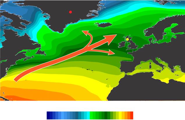
Fig. 1. Surface temperature and heat transport in the North Atlantic Ocean. The relatively mild European climate is sustained by warm sea-surface temperatures and prevailing southwesterly airflow in the North Atlantic Ocean (NAO), with this ameliorating effect being strongest in maritime regions such as Scotland. Mean annual temperature (1979 to present) at 2 m above surface (image obtained using University of Maine Climate Reanalyzer, http://www.cci-reanalyzer.org). Locations of Rannoch Moor and the GISP2 ice core are indicated (yellow and red dots).
Thus the Scottish glacial record is ideal for reconstructing late glacial variability in North Atlantic temperature (Fig. 1). The last glacier resurgence in Scotland—the “Loch Lomond Advance” (LLA)—culminated in a ∼9,500-km2 ice cap centered over Rannoch Moor (Fig. 2A) and surrounded by smaller ice fields and cirque glaciers.
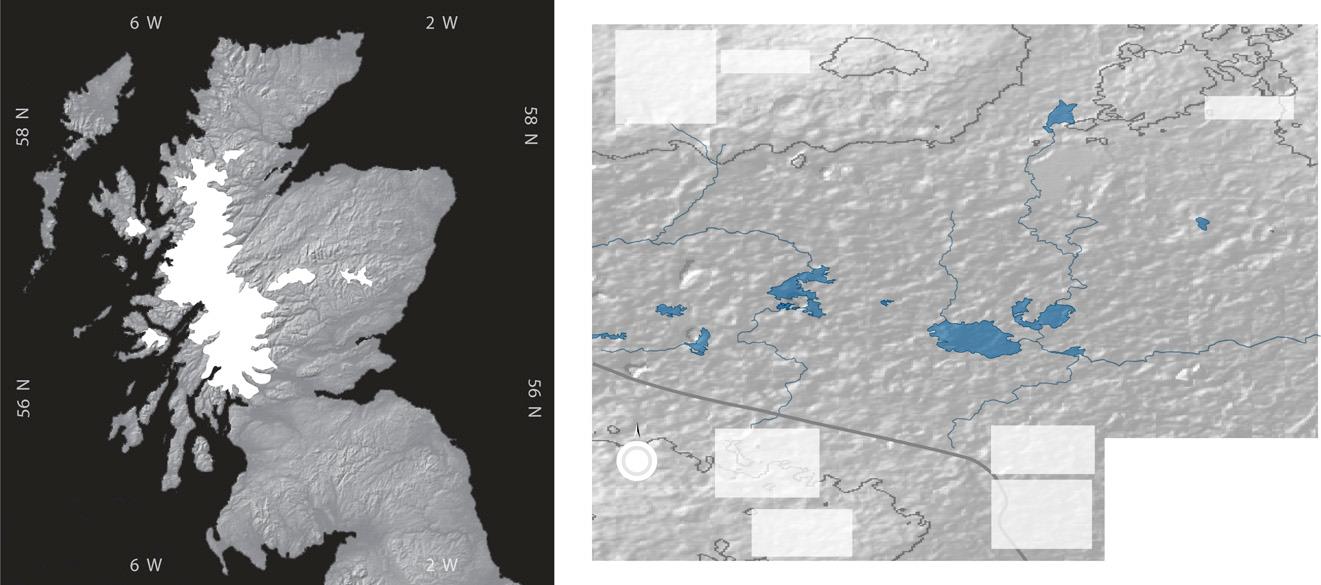
Fig. 2. Extent of the LLA ice cap in Scotland and glacial geomorphology of western Rannoch Moor. (A) Maximum extent of the ∼9,500 km2 LLA ice cap and larger satellite ice masses, indicating the central location of Rannoch Moor. Nunataks are not shown. (B) Glacial-geomorphic map of western Rannoch Moor. Distinct moraine ridges mark the northward active retreat of the glacier margin (indicated by arrow) across this sector of the moor, whereas chaotic moraines near Lochan Meall a’ Phuill (LMP) mark final stagnation of ice. Core sites are shown, including those (K1–K3) of previous investigations (14, 15).
When did the LLA itself occur? We consider two possible resolutions to the paradox of deglaciation during the YDS. First, declining precipitation over Scotland due to gradually increasing North Atlantic sea-ice extent has been invoked to explain the reported shrinkage of glaciers in the latter half of the YDS (18). However, this course of events conflicts with recent data depicting rapid, widespread imposition of winter sea-ice cover at the onset of the YDS (9), rather than progressive expansion throughout the stadial.

Loch Lomond
Furthermore, considering the gradual active retreat of LLA glaciers indicated by the geomorphic record, our chronology suggests that deglaciation began considerably earlier than the mid-YDS, when precipitation reportedly began to decline (18). Finally, our cores contain lacustrine sediments deposited throughout the latter part of the YDS, indicating that the water table was not substantially different from that of today. Indeed, some reconstructions suggest enhanced YDS precipitation in Scotland (24, 25), which is inconsistent with the explanation that precipitation starvation drove deglaciation (26).
We prefer an alternative scenario in which glacier recession was driven by summertime warming and snowline rise. We suggest that amplified seasonality, driven by greatly expanded winter sea ice, resulted in a relatively continental YDS climate for western Europe, both in winter and in summer. Although sea-ice formation prevented ocean–atmosphere heat transfer during the winter months (10), summertime melting of sea ice would have imposed an extensive freshwater cap on the ocean surface (27), resulting in a buoyancy-stratified North Atlantic. In the absence of deep vertical mixing, summertime heating would be concentrated at the ocean surface, thereby increasing both North Atlantic summer sea-surface temperatures (SSTs) and downwind air temperatures. Such a scenario is analogous to modern conditions in the Sea of Okhotsk (28) and the North Pacific Ocean (29), where buoyancy stratification maintains considerable seasonal contrasts in SSTs. Indeed, Haug et al. (30) reported higher summer SSTs in the North Pacific following the onset of stratification than previously under destratified conditions, despite the growing presence of northern ice sheets and an overall reduction in annual SST. A similar pattern is evident in a new SST record from the northeastern North Atlantic, which shows higher summer temperatures during stadial periods (e.g., Heinrich stadials 1 and 2) than during interstadials on account of amplified seasonality (30).
Our interpretation of the Rannoch Moor data, involving the summer (winter) heating (cooling) effects of a shallow North Atlantic mixed layer, reconciles full stadial conditions in the North Atlantic with YDS deglaciation in Scotland. This scenario might also account for the absence of YDS-age moraines at several higher-latitude locations (12, 36–38) and for evidence of mild summer temperatures in southern Greenland (11). Crucially, our chronology challenges the traditional view of renewed glaciation in the Northern Hemisphere during the YDS, particularly in the circum-North Atlantic, and highlights our as yet incomplete understanding of abrupt climate change.
Summary
Several things are illuminated by this study. For one thing, glaciers grow or recede because of multiple factors, not just air temperature. The study noted that glaciers require precipitation (snow) in order to grow, but also melt under warmer conditions. For background on the complexities of glacier dynamics see Glaciermania
Also, paleoclimatology relies on temperature proxies who respond to changes over multicentennial scales at best. C14 brings higher resolution to the table.
Finally, it is interesting to consider climate changing with respect to seasonality. Bromley et al. observe that during Younger Dryas, Scotland shifted from a moderate maritime climate to one with more seasonal extremes like that of inland continental regions. In that light, what should we expect from cooler SSTs in the North Atlantic?
Note also that our modern warming period has been marked by the opposite pattern. Many NH temperature records show slight summer cooling along with somewhat stronger warming in winter, the net being the modest (fearful?) warming in estimates of global annual temperatures.
I’m with Trump on this one: Climate shifts are not a matter of one-way warming, as we have been told.

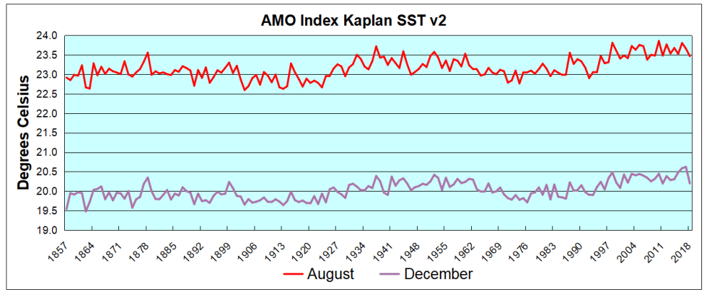
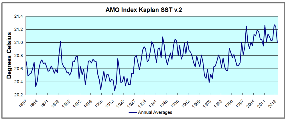
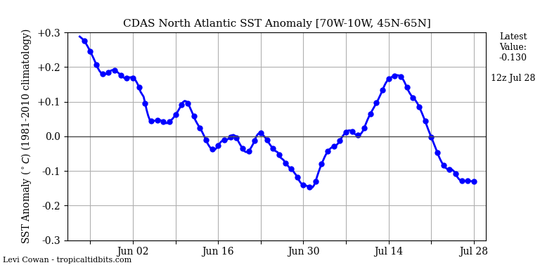
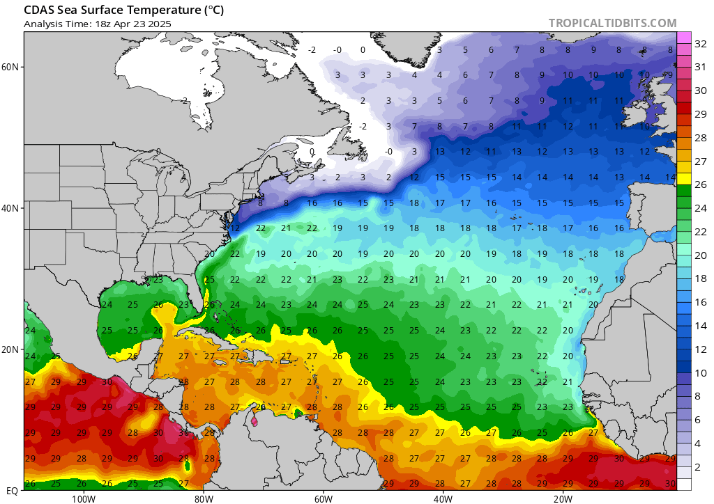
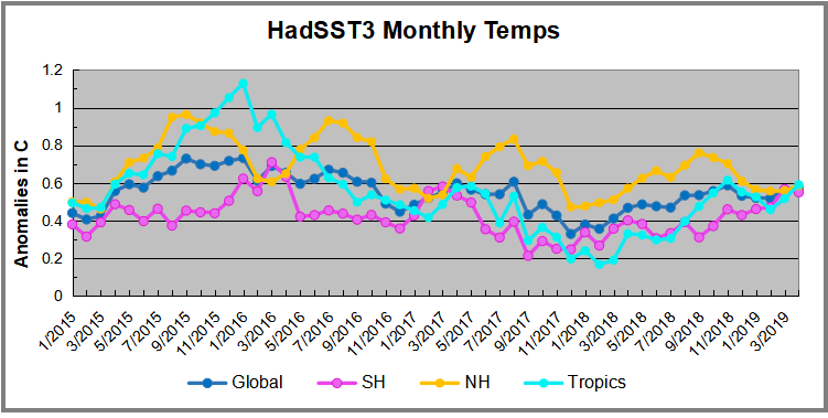
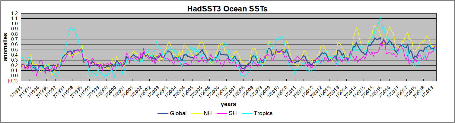
 The best context for understanding decadal temperature changes comes from the world’s sea surface temperatures (SST), for several reasons:


/https://public-media.si-cdn.com/filer/0b/1f/0b1f80a6-748b-405a-a08a-5f35e3a59290/ev115-020.jpg)

