Quantifying Natural Climate Change


Natural climate change

Recent posts have stressed the complexity of climates and their component variables. However, global warming was invented on the back of a single metric: rising global mean temperatures the last decades of last century. That was de-emphasized during the “pause” but re-emerged lately with the El-Nino-induced warming. So this post is focusing on that narrow aspect of climate change.

There are several papers on this blog referring to a quasi-60 year oscillation of surface temperatures due to oceanic circulations. I have also noted the attempts by many to make the link between solar activity (SA) and earth climate patterns.

Dan Pangburn is a professional engineer who has synthesized the solar and oceanic factors into a mathematical model that correlates with Average Global Temperature (AGT). On his blog is posted a monograph (here) Cause of Global Climate Change explaining clearly his thinking and the maths.  I am providing some excerpts and graphs as a synopsis of his analysis, in hopes others will also access and appreciate his work on this issue.

Introduction

The basis for assessment of AGT is the first law of thermodynamics, conservation of energy, applied to the entire planet as a single entity. Much of the available data are forcings or proxies for forcings which must be integrated (mathematically as in calculus, i.e. accumulated over time) to compute energy change. Energy change divided by effective thermal capacitance is temperature change. Temperature change is expressed as anomalies which are the differences between annual averages of measured temperatures and some baseline reference temperature; usually the average over a previous multiple year time period. (Monthly anomalies, which are not used here, are referenced to previous average for the same month to account for seasonal norms.)

At this point, it appears reasonable to consider two temperature anomaly data sets extending through 2015.  These are co-plotted on Figure 8.

Slide8lrg

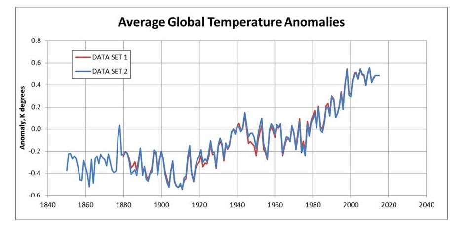
1) The set used previously [12] through 2012 with extension 2013-2015 set at the average 2002-2012 (when the trend was flat) at 0.4864 K above the reference temperature. 2) Current (5/27/16) HadCRUT4 data set [13] through 2012 with 2013-2015 set at the average 2002-2012 at 0.4863 K above the reference temperature.

Accuracy of the model is determined using the Coefficient of Determination, R 2, to compare calculated AGT with measured AGT.

Oceanic Climate Impacts

Approximation of the sea surface temperature anomaly oscillation can be described as varying linearly from –A/2 K in 1909 to approximately +A/2 K in 1941 and linearly back to the 1909 value in 1973. This cycle repeats before and after with a period of 64 years.

Slide1

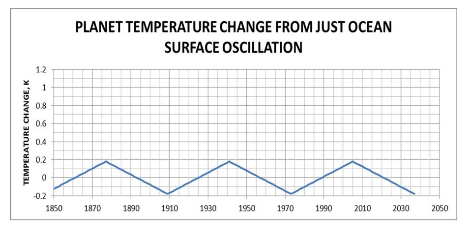
Figure 1: Ocean surface temperature oscillations (α-trend) do not significantly affect the bulk energy of the planet.

Comparison with PDO, ENSO and AMO

Ocean cycles are perceived to contribute to AGT in two ways: The first is the direct measurement of sea surface temperature (SST). The second is warmer SST increases atmospheric water vapor which acts as a forcing and therefore has a time-integral effect on temperature. The approximation, (A,y), accounts for both ways.

Successful accounting for oscillations is achieved for PDO and ENSO when considering these as forcings (with appropriate proxy factors) instead of direct measurements. As forcings, their influence accumulates with time. The proxy factors must be determined separately for each forcing.

Slide2

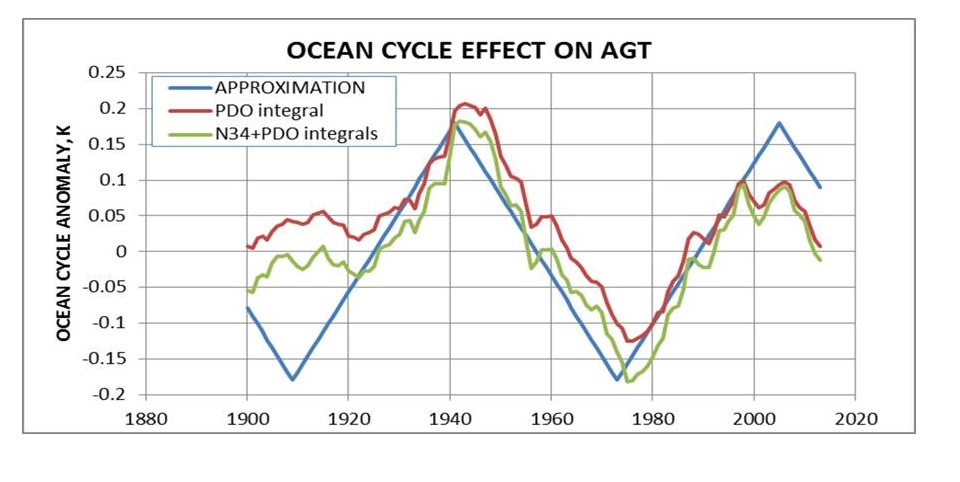
Figure 2: Comparison of idealized approximation of ocean cycle effect and the calculated effect from PDO and ENSO.

The AMO index [9] is formed from area-weighted and de-trended SST data. It is shown with two different amounts of smoothing in Figure 3 along with the saw-tooth approximation for the entire planet per Equation (2) with A = 0.36.

Slide3

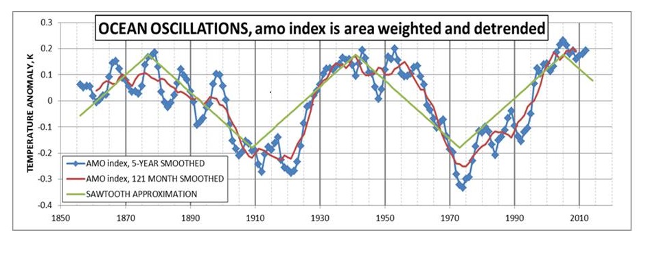
The high coefficients of determination in Table 1 and the comparisons in Figures 2 and 3 corroborate the assumption that the saw-tooth profile with a period of 64 years provides adequate approximation of the net effect of all named and unnamed ocean cycles in the calculated AGT anomalies.

Solar-Climate Connection

An assessment of this is that sunspots are somehow related to the net energy retained by the planet, as indicated by changes to average global temperature. Fewer sunspots are associated with cooling, and more sunspots are associated with warming. Thus the hypothesis is made that SSN are proxies for the rate at which the planet accumulates (or loses) radiant energy over time. Therefore the time-integral of the SSN anomalies is a proxy for the amount of energy retained by the planet above or below breakeven.

Also, a lower solar cycle over a longer period might result in the same increase in energy retained by the planet as a higher solar cycle over a shorter period. Both magnitude and time are accounted for by taking the time-integral of the SSN anomalies, which is simply the sum of annual mean SSN (each minus Savg) over the period of study.

The values for Savg are subject to two constraints. Initially they are determined as that which results in derived coefficients and maximum R2. However, calculated values must also result in rational values for calculated AGT at the depths of the Little Ice Age. The necessity to calculate a rational LIA AGT is a somewhat more sensitive constraint. The selected values for Savg result in calculated LIA AGT of approximately 1 K less than the recent trend which appears rational and is consistent with most LIA AGT assessments.

The sunspot number anomaly time-integral is a proxy for a primary driver of the temperature anomaly β-trend. By definition, energy change divided by effective thermal capacitance is temperature change.

Slide10

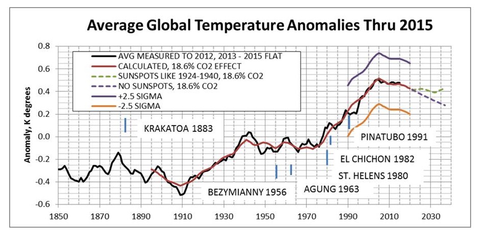
Figure 10: 5-year running average of measured temperatures with calculated prior and future trends (Data Set 1) using 34 as the average daily sunspot number and with V1 SSN. R2 = 0.978887

Projections until 2020 use the expected sunspot number trend for the remainder of solar cycle 24 as provided [6] by NASA. After 2020 the ‘limiting cases’ are either assuming sunspots like from 1924 to 1940 or for the case of no sunspots which is similar to the Maunder Minimum.

Some noteworthy volcanoes and the year they occurred are also shown on Figure 9. No consistent AGT response is observed to be associated with these. Any global temperature perturbation that might have been caused by volcanoes of this size is lost in the natural fluctuation of measured temperatures.

Although the connection between AGT and the sunspot number anomaly time-integral is demonstrated, the mechanism by which this takes place remains somewhat speculative.

Various papers have been written that indicate how the solar magnetic field associated with sunspots can influence climate on earth. These papers posit that decreased sunspots are associated with decreased solar magnetic field which decreases the deflection of and therefore increases the flow of galactic cosmic rays on earth.

These papers [14,15] associated the increased low-altitude clouds with increased albedo leading to lower temperatures. Increased low altitude clouds would also result in lower average cloud altitude and therefore higher average cloud temperature. Although clouds are commonly acknowledged to increase albedo, they also radiate energy to space so increasing their temperature increases S-B radiation to space which would cause the planet to cool. Increased albedo reduces the energy received by the planet and increased radiation to space reduces the energy of the planet. Thus the two effects work together to change the AGT of the planet.

Summary

Simple analyses [17] indicate that either an increase of approximately 186 meters in average cloud altitude or a decrease of average albedo from 0.3 to the very slightly reduced value of 0.2928 would account for all of the 20th century increase in AGT of 0.74 K. Because the cloud effects work together and part of the temperature change is due to ocean oscillation (low in 1901, 0.2114 higher in 2000), substantially less cloud change would suffice.

All of this leaves little warming left to attribute to rising CO2. Pangburn estimates CO2 forcing could be at most 18.6% or 0.23C added since 1895. Given uncertainties in proxies from the past, the estimate could be as low as 0.05C, and the correlation with natural factors would still be .97 R2.

However, all is not lost for CO2. It is still an important player in the atmosphere, despite its impotence as a warming agent.


Climate Partly Cloudy

Dr. Curry has a new very informative post (here) on clouds and climate, including links to several studies recently announced from CERN and others. It reminded me of Joni Mitchell’s song Both Sides Now:

Bows and flows of angel hair
And ice cream castles in the air
And feather canyons everywhere
I’ve looked at clouds that way
But now they only block the sun
They rain and snow on everyone
So many things I would have done
But clouds got in my way

I’ve looked at clouds from both sides now
From up and down and still somehow
It’s clouds’ illusions I recall
I really don’t know clouds at all
– Joni Mitchell – Both Sides Now Lyrics

The above chorus could serve as an anthem for climate modelers. Clouds are arguably the least understood and most unpredictable of factors in climate change. We are getting much better at the weather connection between storms and cloud formation. But the long-term effects of clouds and cloudiness are still uncertain. Dr. Curry helpfully separates the cloud problem into two issues: cloud microphysics and cloud dynamics. She observes that the latter is much more difficult and also has much more impact on climate.

Some things are known and described in textbooks of Atmospheric Physics. In introducing Chapter 9: Aerosols and Clouds in his updated volume, Murray Salby (here) suggests the complexities involved:

Radiative transfer is modified importantly by cloud. Owing to its high reflectivity in the visible, cloud shields the Earth-atmosphere system from solar radiation. It therefore introduces cooling in the SW energy budget of the Earth’s surface, offsetting the greenhouse effect. Conversely, the strong absorptivity in the IR of water and ice sharply increases the optical depth of the atmosphere. Cloud thus introduces warming in the LW energy budget of the Earth’s surface, reinforcing the greenhouse effect. We develop cloud processes from a morphological description of atmospheric aerosol, without which cloud would not form. The microphysics controlling cloud formation is then examined. Macrophysical properties of cloud are developed in terms of environmental conditions that control the formation of particular cloud types. These fundamental considerations culminate in descriptions of radiative and chemical processes that involve cloud.

Cloud Formation

The microphysics is mostly related to how clouds form, and the role of aerosols. Even though clouds can form simply from enough water vapor, in practice the required conditions for such “homogenous” formation are higher than those needed for “heterogenous” formation from ever-present aerosols, termed CCN. From Salby (pg. 272):

The simplest means of forming cloud is through homogeneous nucleation, wherein pure vapor condenses to form droplets. . . Yet, the formation of most cloud cannot be explained by homogeneous nucleation. Instead, cloud droplets form through heterogeneous nucleation, wherein water vapor condenses onto existing particles of atmospheric aerosol. Termed cloud condensation nuclei (CCN), such particles support condensation at supersaturations well below those required for homogeneous nucleation.

Cloudiness Impact on Radiative Balance

The extent of cloudiness varies a lot, as shown by measures of OLR (Outgoing Longwave Radiation) by satellites above TOA (h/t greensand). Notice that the scale has a range of 100 W m^2 compared to estimated CO2 sensitivity of ~4 W m^2.

OLR or ‘Cloudiness’ at the equatorial dateline 7.5S – 7.5N, 170E – 170W (large sea surface area) has been below norm for 15/16 months. Below average OLR is the result of increased cloud cover, which in turn = reduced insolation, less incoming solar energy. Yet as Salby says, cloud tops can reflect SW solar energy away while the cloud mass absorbs IR from the surface, delaying cooling. Different types of clouds have different impacts on radiative forcing. Not to mention water changing between all 3 phases inside.

Therein lies the cloud conundrum: How much warming and how much cooling from changes in cloudiness?

giphy

Clouds Complicating Climate
Salby, 9.5.1.pg.315ff

A quantitative description of how cloud figures in the global energy budget is complicated by its dependence on microphysical properties and interactions with the surface. These complications are circumvented by comparing radiative fluxes at TOA under cloudy vs clear-sky conditions. Over a given region, the column-integrated radiative heating rate must equal the difference between the energy flux absorbed and that emitted to space.

Shortwave cloud forcing represents cooling. It is concentrated near the Earth’s surface, because the principal effect of increased albedo is to shield the ground from incident SW. Longwave cloud forcing represents warming. It is manifest in heating near the base of cloud and cooling near its top (Fig. 9.36b).

That radiative forcing depends intrinsically on the vertical distribution of cloud. For instance, deep cumulonimbus and comparatively shallow cirrostratus can have identical cloud-top temperature, yielding the same LW forcing of the TOA energy budget. However, they have very different optical depths, producing very different vertical distributions of radiative heating. The strong correlation between water vapor and cloud cover introduces another source of uncertainty.

Summary

Since 90% of water in the atmosphere comes from the ocean, clouds are another way that Oceans Make Climate. And as Roger Andrews demonstrates (here) cloudiness correlates quite positively with SSTs.

Bottom Line: Any CO2 effect is lost in the Clouds

Globally averaged values of CLW and CSW are about 30 and −45 W m−2, respectively. Net cloud forcing is then −15 W m−2. It represents radiative cooling of the Earth atmosphere system. This is four times as great as the additional warming of the Earth’s surface that would be introduced by a doubling of CO2. Latent heat transfer to the atmosphere (Fig. 1.32) is 90 W m−2. It is an order of magnitude greater. Consequently, the direct radiative effect of increased CO2 would be overshadowed by even a small adjustment of convection (Sec. 8.7).


Ocean Trumps Global Warming

Internal Climate Variability Trumps Global Warming (here) is a
great post by hydrologist Rob Ellison confirming how the Oceans Make Climate. He was intrigued by discovering that rivers in eastern Australia changed form – from low energy meandering to high energy braided forms and back – every few decades. For almost 30 years he looked for the source and import of this variability, and has found it in the ocean.

Turns out that it is a combination of conditions in the northern and central Pacific Ocean that is of immense significance. A 20 to 30 year change in the volume of frigid and nutrient rich water upwelling from the abysmal depths. A generally warmer or cooler sea surface in the northern Pacific and greater frequency and intensity of El Niño or La Niña respectively. This sets up changes in patterns of wind, currents and cloud that cause changes in rainfall, biology and temperature globally. In the cool pattern shown above – booming ecologies, drought in the Americas and Europe, rainfall in Australia, Indonesia, Africa, China and India and cooler global temperatures. The reverse in the warm phase. Warming to 1944, cooling to 1976, warming again to 1998 and – at the least – not warming since. It leads to a prediction that the La Niña currently emerging is likely to be large.

A Persistent Ocean Cycle

Changes in the Pacific Ocean state can be traced in sediment, ice cores, stalagmites and corals. A record covering the last 12,000 years was developed by Christopher Moy and colleagues from measurements of red sediment in a South American lake. More red sediment is associated with El Niño. The record shows periods of high and low El Niño activity alternating with a period of about 2,000 years. There was a shift from La Niña dominance to El Niño dominance 5000 years ago that is associated with the drying of the Sahel. There is a period around 3,500 years ago of high El Niño activity associated with the demise of the Minoan civilisation (Tsonis et al, 2010).

Tessa Vance and colleagues devised a 1000 year record from salt content in an Antarctic ice core. More salt is La Niña as a result of changing winds in the Southern Ocean. It revealed several interesting facts. The persistence of the 20 to 30 year pattern. A change in the period of oscillation between El Niño and La Niña states at the end of the 19th century. A 1000 year peak in El Niño frequency and intensity in the 20th century which resulted in uncharacteristically dry condition since 1920.

Conclusion

The whole post is worth reading and a solid contribution to our understanding. Ellison’s summary is pertinent, compelling and wise.

It is quite impossible to quantify natural and anthropogenic warming in the 20th century.  The assumption that it was all anthropogenic is quite wrong.  The early century warming was mostly natural – as was at least some of the late century warming.  It seems quite likely that a natural cooling with declining solar activity – amplified through Pacific Ocean states – will counteract rather than add to future greenhouse gas warming.   A return to the more common condition of La Niña dominance – and enhanced rainfall in northern and eastern Australia – seems more likely than not.

I predict – on the balance of probabilities – cooler conditions in this century.  But I would still argue for returning carbon to agricultural soils, restoring ecosystems and research on and development of cheap and abundant energy supplies.  The former to enhance productivity in a hungry world, increase soil water holding capacity, improve drought resilience, mitigate flooding and conserve biodiversity.  We may in this way sequester all greenhouse gas emissions for 20 to 30 years.  The latter as a basis for desperately needed economic growth.  Climate change seems very much an unnecessary consideration and tales of climate doom – based on wrong science and unfortunate policy ambitions – a diversion from practical and measured development policy.

Australia’s River Systems ABC

Cutting Edge Sea Level Data


PSLMPThis post is about the SEAFRAME network measuring sea levels in the Pacific, and about the difficulty to discern multi-decadal trends of rising or accelerating sea levels as evidence of climate change.

Update May 10 below, regarding recent Solomon Islands news

Pacific Sea Level Monitoring Network

The PSLM project was established in response to concerns voiced by Pacific Island countries about the potential effects of climate change. The project aims to provide an accurate long-term record of sea levels in the area for partner countries and the international scientific community, and enable the former to make informed decisions about managing their coastal environments and resources.

In 1991, the National Tidal Facility (NTF) of the Flinders University of South Australia was awarded the contract to undertake the management of the project.  Between July 1991 and December 2000 sea level and meteorological monitoring stations were installed at 11 sites. Between 2001 and 2005 another station was established in the Federated States of Micronesia and continuous global positioning systems (CGPS) were installed in numerous locations to monitor the islands’ vertical movements.

The 14 Pacific Island countries now participating in the project provide a wide coverage across the Pacific Basin: the Cook Islands, Federated States of Micronesia, Fiji, Kiribati, Marshall Islands, Nauru, Niue, Palau, Papua New Guinea, Samoa, Solomon Islands, Tonga, Tuvalu and Vanuatu.

SPSLCM_2008_4_data_report_Image_11

Each of these SEA Level Fine Resolution Acoustic Measuring Equipment (SEAFRAME) stations in the Pacific region are continuously monitoring the Sea Level, Wind Speed and Direction, Wind Gust, Air and Water Temperatures and Atmospheric Pressure.

In addition to its system of tide gauge facilities, the Pacific Sea-Level Monitoring Network also includes a network of earth monitoring stations for geodetic observations, implemented and maintained by Geoscience Australia. The earth monitoring installations provide Global Navigation Satellite System (GNSS) measurements to allow absolute determination of the vertical height of the tide gauges that measure sea level.

Sea Level Datasets from PSLM

Data and reports are here.

Monthly reports are detailed and informative. At each station water levels are measured every six minutes in order to calculate daily maxs, mins and means, as a basis for monthly averages. So the daily mean sea level value is averaged from 240 readings, and the daily min and max are single readings taken from the 240.


untitled

A typical monthly graph appears above. It shows how tides for these stations range between 1 to 3 meters daily, as well variations during the month.

According to the calibrations, measurement errors are in the range of +/- 1 mm. Vertical movement of the land is monitored relative to a GPS benchmark. So far, land movement at these stations has also been within the +/- 1 mm range (with one exception related to an earthquake).

The PSLM Record

March SL range

In the Monthly reports are graphs showing results of six minute observations, indicating tidal movements daily over the course of a month.The chart above shows how sea level varied in each location during March 2016 compared to long term March results. Since many stations were installed in 1993, long term means about 22 years of history.

This dataset for Pacific Sea Level Monitoring provides a realistic context for interpreting studies claiming sea level trends and/or acceleration of such trends. Of course, one can draw a line through any scatter of datapoints and assert the existence of a trend. And the error ranges above allow for annual changes of a few mm to be meaningful. Here is a table produced in just that way.

Location Installation date Sea-level trend (mm/yr)
Cook Islands Feb 2003 +5.5
Federated States of Micronesia Dec 2001 +17.7
Fiji Oct 1992 +2.9
Kiribati Dec 1992 +2.9
Marshall Islands May 1993 +5.2
Nauru Jul 1993 +3.6
Papua New Guinea Sept 1994 +8.0
Samoa Feb 1993 +6.9
Solomon Islands Jul 1994 +7.7
Tonga Jan 1993 +8.6
Tuvalu Mar 1993 +4.1
Vanuatu Jan 1993 +5.3

The rising trends range from 2.9 to 8.6 mm/year (FSM is too short to be meaningful).

Looking into the details of the monthly anomalies, it is clear that sea level changes at the mm level are swamped by volatility of movements greater by orders of magnitude.  And there are obvious effects from ENSO events. The 1997-98 El Nino shows up in a dramatic fall of sea levels almost everywhere, and that event alone creates most of the rising trends in the table above.  The 2014-2016 El Nino is also causing sea levels to fall, but is too recent to affect the long term trend.

Picture17revSummary

Sea Level Rise is another metric for climate change that demonstrates the difficulty discerning a small change of a few millimeters in a dataset where tides vary thousands of millimeters every day. And the record is also subject to irregular fluctuations from storms, currents and oceanic oscillations, such as the ENSO.

On page 8 of its monthly reports (here), PSLM project provides this caution regarding the measurements:

The overall rates of movement are updated every month by calculating the linear slope during the tidal analysis of all the data available at individual stations. The rates are relative to the SEAFRAME sensor benchmark, whose movement relative to inland benchmarks is monitored by Geosciences Australia.
Please exercise caution in interpreting the overall rates of movement of sea level – the records are too short to be inferring long-term trends.

A longer record will bring more insight, but even then sea level trends are a very weak signal inside a noisy dataset. Even with state-of-the-art equipment, it is a fool’s errand to discern any acceleration in sea levels, in order to link it to CO2. Such changes are in fractions of millimeters when the measurement error is +/- 1 mm.

For more on the worldwide network of tidal gauges, as well as satellite systems attempting to measure sea level, sea Dave Burton’s excellent website.

May 10 update Regarding recent news about Solomon Islands.

As the charts above show, there is negligible sea level rise in the West Pacific, and receding a bit lately at Solomon Islands.  So it was curious that the media was declaring those islands inundating because of climate change.

Now the real story is coming out (but don’t wait for the retractions)

A new study published in Environmental Research Letters shows that some low-lying reef islands in the Solomon Islands are being gobbled up by “extreme events, seawalls and inappropriate development, rather than sea level rise alone.” Despite headlines claiming that man-made climate change has caused five Islands (out of nearly a thousand) to disappear from rising sea levels, a closer inspection of the study reveals the true cause is natural, and the report’s lead author says many of the headlines have been ‘exaggerated’ to ill-effect.

http://www.examiner.com/article/sinking-solomon-islands-and-climate-link-exaggerated-admits-study-s-author


Atlantic Ocean Cooling

Most oceanographers have noted quasi-60-year cycles in warming and cooling of the oceans, with offsets between Pacific and Atlantic.  Thus it has been expected that early this century the oceanic temperature regime should shift from the warming phase that dominated the 1980s to 2000.

Paul Dorian at Vencore Weather has an excellent post (here) showing how this cooling regime is in process in the Atlantic.  By several measures, the cooling is evident and likely to be a long term (decadal or more) phenomenon.

From his Overview:

In general, the Atlantic Ocean experienced a cold phase from the early 1960’s to the mid 1990’s at which time it flipped to a warm phase and that has continued for the most part ever since. The current warm phase; however, is now showing signs of a possible long-term shift back to colder-than-normal sea surface temperatures (SST) and this could have serious implications on US climate and sea ice areal extent in the Northern Hemisphere.

His charts show the transition is underway, with the warming peak around 2007.

And as has been noted on this blog (here) regarding Arctic sea ice, the decline went flat after 2007.

Summary

The oceans make climate, and the future looks more like cooling than warming.


Dr. Arnd Bernaerts Disappeared

As happened in Soviet Russia, Climate revisionists are rewriting history. Judith Curry was one of 20 leading climate scientists according to the “Climate Council” based in Australia. But in March 2016, the list was reduced to 19, and Dr Curry disappeared (here).

Now the biography of Arnd Bernaerts has disappeared from Wikipedia, despite his obvious contributions to ocean science and law. UN Undersecretary-General Satya N. Nandan: “Mr Bernaerts has given to the international community an invaluable guide to the understanding and implementation of the 1982 United Nations Convention on the Law of the Sea.” (1988).

Most likely the revisionists are unhappy with Bernaerts’ coining of phrases such as these:

Climate is the continuation of oceans by other means.

Oceans govern climate.

And his writings are extensive and contemporary, as noted on this blog under the category Oceans Make Climate, inspired by my discovery of his work:
https://rclutz.wordpress.com/2015/04/07/oceans-matter-reflecting-on-writings-by-dr-arnd-bernaerts/

You can do something against the efforts of alarmists such as William Connolley by responding to Dr. Bernaerts here.

The Deleted Biography is here.

Man Made Mild Weather (MMMW)

For some relief from the relentless stories of Catastrophic Anthropogenic Global Warming (CAGW), we turn today to a study of Man Made Mild Weather (MMMW).  CAGW also stands for Citizens Against Government Waste, not to be confused with the first acronym.  Oh wait.  (sarc/off)

Specifically this post concerns work by Dr. Arnd Bernaerts on human activities contributing to mild winters in Europe.

To start with, he is analyzing “climate” properly. Climates are plural, not singular; the term is a human construct referring to distinctly local and regional patterns and expectations of future weather. Secondly, he addresses changes observed in one particular season as a way to identify inter annual variation. Thirdly, he is well aware of oceanic fluctuations, and seeks to understand human effects in addition to natural variability.

Specifically Dr. Bernaerts studies the linkage between the Baltic and North Seas and winters in Northern Europe. His article (here) is entitled “Northern Europe’s Mild Winters. Contributions from Offshore Industry, Ships, Fishery, et cetera?”

From the Abstract:
The marine environment of North Sea and Baltic is one of the most heavily strained by numerous human activities. Simultaneously water and air temperatures increase more than elsewhere in Europe and globally, which cannot be explained with ‘global warming’.

The climatic change issue would be better understood if this extraordinary regional warming is sufficiently explained. The regional features are unique for in-depth studies due to different summer-winter conditions, shallowness of the seas, geographical structure, and main pathway for maritime weather patterns moving eastwards.

The impact of sea activities on the seasonal sea water profile structure is contributing to stronger regional warming, change in growing season, and less severe sea ice conditions. The impact of the man, whether small or large, should be understood very soon and very thoroughly.

Pay particular attention to the Discussion at the end, which includes this:

Regional seas in Northern Europe are minor from size and volume in global ocean affairs. Weather is “done” elsewhere, but every location contributes to the global picture. In the case of N-Europe it may be more significant as weather can be divided in maritime and continental influence, and due to the global air circulation from West to East, it is a gate. It may support the flow of warm wet air eastward (low pressure), or stem it by dry and cold continental air (high pressure), by diverting low pressure areas– in extreme circumstances – towards the Bering Sea or Mediterranean. In so far the North Sea and Baltic play a crucial role in how to open or close this gate.

Three facts are established: higher warming, a small shift in the seasons, and a decreasing sea ice cover. In each scenario the two sea’s conditions play a decisive role. These conditions are impaired by wind farms, shipping, fishing, off shore drilling, under sea floor gas-pipe line construction and maintenance, naval exercise, diving, yachting, and so on, about little to nothing has been investigated and is understood.

Summary:
The facts are conclusive. ‘Global Climate Change’ cannot cause a special rise in temperatures in Northern Europe, neither in the North Sea nor the Baltic or beyond. Any use of the oceans by mankind has an influence on thermo-haline structures within the water column from a few cm to 10m and more. Noticeable warmer winters in Europe are the logical consequence

Conclusion:

Two of my heroes are Dr. Pielke Sr. for his work showing how human use of the land affects climates in the locales where it occurs, and Dr. Bernaerts for exposing how human use of the ocean impacts on nearby climates.

Man-Made Ocean Warming? Yes, but it’s not CO2.

Forecasted Temperature anomalies 2 meters above ground for February 2016 in Europe


Dr Arnd Bernaerts has long studied effects in Northern European Seas. Here are excerpts from his recent publication: Offshore Wind-Parks and Northern Europe’s Mild Winters: Contribution from Ships, Fishery, et cetera? http://www.davidpublisher.org/Public/uploads/Contribute/569da5d061f90.pdf

His main point from the abstract: The marine environment of North Sea and Baltic is one of the most heavily strained by numerous human activities. Simultaneously water and air temperatures increase more than elsewhere in Europe and globally, which cannot be explained with “global warming”.

Excerpts:

Since mankind, during the course of a year, agitates the water column of North Sea and Baltic by stirring, more warmth is taken to deeper water in the summer season and rises to the surface from lower layers in the winter period, where heat is exchanged with the air until sea icing is observed. This is a process that can be seen from the beginning of September until the end of March.

Marine activities play a much bigger role in time factor and duration of ice formation. If the sea surface temperature has already reached the freezing point, any vessel shovels warmer water to the surface, or vice versa, forcing a more rapid melt… The shrinking ice cover correlates well with an increase in human activities, and subsequently leading to higher air temperature throughout the region.

Basically three facts are established: higher warming, a small shift in the seasons, and a decreasing sea ice cover. In each scenario the two seas’ conditions play a decisive role (North Sea and Baltic). These conditions are impaired by wind farms, shipping, fishing, off shore drilling, under sea floor gas-pipe line construction and maintenance, naval exercise, diving, yachting, and so on, about little to nothing has been investigated and is understood.

Summary
The facts are conclusive. “Global Climate Change” cannot cause a special rise in temperatures in Northern Europe, neither in the North Sea nor the Baltic or beyond. Any use of the oceans by mankind has an influence on thermo-haline structures within the water column from a few cm to 10m and more. Noticeable warmer winters in Europe are the logical consequence.

North Americans should not think themselves unaffected by all this.
Consider this graphic of the Siberian Express:

The more the Atlantic weather governs the situation beyond the Ural the further Polar and Siberian cold will be pushed eastwards, called ‘Siberian Express’(Fig.10). This was felt in Alaska, Canada and Eastern U.S. Many days were extremely cold with deviations from the mean of 20°C and beyond.

More information is here:

http://www.ocean-climate-law.com/12/arch/12.html

Barents Icicles

A chart of Barents Ice Cycles looks a lot like the icicles above, except upside down since Barents Sea is usually all water by September. Notice the black lines in the graph below hitting bottom near zero.

Note also the anomalies in red are flat until 1998, then decline to 2007 and then flat again.

Why Barents Sea Ice Matters

Barents Sea is No. 1, being located at the gateway between the Arctic and North Atlantic. Previous posts (here and here) have discussed research suggesting that changes in Barents Sea Ice may signal changes in Arctic Sea Ice a few years later. As well, the studies point to changes in heat transport from the North Atlantic driving the Barents Sea Ice, along with changes in salinity of the upper layer. And, as suggested by Zakharov (here), there are associated changes in atmospheric circulations, such as the NAO (North Atlantic Oscillation).

Here we look at MASIE over the last decade and other datasets over longer terms in search for such patterns.

Observed Barents Sea Ice

Below is a more detailed look at recent years.

Barents Masierrev

This graph shows that the last two years were outliers in opposite directions. 2014 was an exceptionally high annual average due to melting delayed until April, and then a much higher minimum and faster than average recovery. In contrast 2015 was high initially, became average by day 91, then dropped sharply to a meltout, followed by a slower recovery. 2012 shows the lowest Barents ice year contrasting with 2014, the highest annual extent in the last decade.

Annual average BSIE (Barents Sea Ice Extent) is 315k km2, varying between 250k and 400k over the last ten years. The volatility is impressive, considering the daily Maximums and Minimums in the record. Average Max is 781k, ranging from 608k to 936k. Max occurs on day 77 (average) with a range from day 36 to 103. Average Min is 11k on day 244, ranging from 0k to 77k, and from days 210 to 278.

In fact, over this decade, there are not many average years. Five times BSIE melted to zero, two were about average, and 3 years much higher: 2006-7 were 2 and 3 times average, and 2014 was 7 times higher at 77k.

As for Maxes, only 1 year matched the 781k average. Four low years peaked at about 740k (2006,07,08 and 14), and the lowest year at 608k (2012). The four higher years start with the highest one, 936k in 2010, and include 2011, 13, and 15.

Comparing Barents Ice and NAO
Barents Masierev

This graph confirms that Barents winter extents (JFMA) correlate strongly (0.73) with annual Barents extents. And there is a slightly less strong inverse correlation with NAO index (-0.64). That means winter NAO in its negative phase is associated with larger ice extents, and vice-versa.

Comparing Barents Ice and Arctic Annual

Barents and Arctic

Arctic Annual extents correlate with Barents Annuals at a moderately strong 0.46, but have only weaker associations with winter NAO or Barents winter averages. It appears that 2012 and 2015 interrupted a pattern of slowly rising extents.

NAO and Arctic Ice Longer Term

Fortunately there are sources providing an history of Arctic ice longer term and overlapping with the satellite era. For example:

Observed sea ice extent in the Russian Arctic, 1933–2006 Andrew R. Mahoney et al (2008)
http://seaice.alaska.edu/gi/publications/mahoney/Mahoney_2008_JGR_20thC_RSI.pdf

Russian Arctic Sea Ice to 2006

Mahoney et al say this about Arctic Ice oscillations:

We can therefore broadly divide the ice chart record into three periods. Period A, extending from the beginning of the record until the mid-1950s, was a period of declining summer sea ice extent over the whole Russian Arctic, though not consistently in every individual sea. . . Period B extended from the mid-1950s to the mid- 1980s and was a period of generally increasing or stable summer sea ice extent. For the Russian Arctic as a whole, this constituted a partial recovery of the sea ice lost during period A, though this is not the case in all seas. . . Period C began in the mid-1980s and continued to the end of the record (2006). It is characterized by a decrease in total and MY sea ice extent in all seas and seasons.

Comparing Arctic Ice with winter NAO index

The standardized seasonal mean NAO index during cold season (blue line) is constructed by averaging the monthly NAO index for January, February and March for each year. The black line denotes the standardized five-year running mean of the index. Both curves are standardized using 1950-2000 base period statistics.

The graph shows roughly a 60 year cycle, with a negative phase 1950-1980 and positive 1980 to 2010. As described above, Arctic ice extent grew up to 1979, the year satellite ice sensing started, and declined until 2007. The surprising NAO uptick recently coincides with the anomalous 2012 and 2015 meltings.

As of January 2016 NAO has gone negative for the first time in months.

Summary

If the Barents ice cycle repeats itself over the next decades, we should expect Arctic ice extents to grow as part of a natural oscillation. The NAO atmospheric circulation pattern is part of an ocean-ice-atmosphere system which is driven primarily by winter changes in the North Atlantic upper water layer.

Self-Oscillating Sea Ice System

Self-Oscillating Sea Ice System  See here.


Arctic Sea Ice: Self-Oscillating System

The Climate System is Self-Oscillating: Sea Ice Proves It.

Scientists have studied the Arctic for a long time at the prestigious AARI: Arctic and Antarctic Research Institute St. Petersburg, Russia. V. F. Zakharov has published a complete description supported by research findings under this title: Sea Ice In the Climate System A Russian View (here)

Below I provide excerpts from this extensive analysis to form a synopsis of their view: Component parts of the climate system interact so that Arctic Sea Ice varies within a range constrained by those internal forces.

Self-Oscillating Sea Ice System

Self-Oscillating Sea Ice System

The most probable regulator of the physical geographical process can be found from analysis of the relationships between the components of the climate system. It is not necessary to investigate the cause-effect relationships between all these components in succession. It is sufficient to choose one of them, let us say sea ice, and consider its direct interaction with the atmosphere and the ocean – in the climate system and the significance of internal mechanisms in the natural process. Pg 1

The idea that the ice area growth at present can be achieved by changes in only the haline structure of the upper ocean layer, as a result of surface Arctic water overflowing onto warmer but more saline water, is supported both by calculations and empirical data. Pg. 46

First of all, it should be noted that the signs of temperature and salinity anomalies coincide in most cases: a decreased salinity corresponds to enhanced temperature and vice versa. Such similarity in the change of these parameters is impossible to explain from the point of view of the governing role of thermal conditions in the atmosphere with regard to the ocean, as the air temperature increase and decrease can result only in the change of the thermal state of sea surface layer not its salinity. Pgs. 48-49

Thus, the presented facts suggest that the most significant cause of changes in the ice cover extent are the changes in the vertical water structure in the upper ocean layer, rather than the changes of thermal conditions in the atmosphere. These changes are induced by fluctuations in the horizontal dimensions of the halocline, which are governed in turn by the expansion or reduction of the surface Arctic water mass. Pg. 49

It follows from the above that, under present day conditions, the changes in the area of the Arctic sea ice during the colder period of the year can be induced only by the change in the haline structure of the upper ocean layer. Indirectly, this change will also affect the thermal state of the atmosphere. Pg. 56

It is important to note that the ice effect on the atmosphere is not limited to the thermal effect. That it can produce a significant effect on atmospheric circulation is already evident from the fact that the Arctic anticyclone, considered by Viese [13] as a regulator of atmospheric processes in the Northern polar region, could form as a pressure formation only in the conditions of the ice regime in the Arctic. Pg. 56


Zacharov fig.24

Zakharov fig.24

An analysis of cause-effect relationships does not leave any doubt in what direction and in what order the climate signal propagates in the atmosphere-ocean-polar ice system. This is not the direction and order usually assumed to cause present climate change. When it has become clear that the changes in the ocean, caused by disturbances of its freshwater balance, precede changes in the extent of sea ice, and the latter the changes in the atmosphere, then there was nothing left but for us to acknowledge self oscillation to be the most probable explanation for the development of the natural process. Pg. 58

Maybe the most convincing evidence of the Arctic sea ice stability is its preservation during the last 700,000 years despite vast glacial- interglacial fluctuations. The surface air temperature in the Arctic during the interglacial periods was higher by several degrees than present day temperatures. Pg. 44

Conclusion:

The remarkable stability of our planetary climate system derives from feedbacks between internal parts of the system, providing the oscillations we observe as natural variability. Arctic Sea Ice is a prime example.