E.M. Smith (Chiefio) has new post (here) presenting the evidence showing how Nitrogen, the dominant gas in the atmosphere, also radiates in the infrared, and thus participates in the “greenhouse” effect. This information was measured and reported as long ago as 1944, but the implications have been ignored in the recent obsession with CO2.
This Changes Everything.
Footnote: The original discovery of this effect from Nitrogen (here) attributes the IR to N atoms present in the upper atmosphere.
People are duped by false alarms about Arctic sea ice because they have (subliminally) bought into the notion likening the Arctic to their home refrigerator. This post is to dissuade you from taking on board that false analogy.
Inside Your Fridge
When you put liquid water into your fridge, it releases heat, both sensible and latent, the air in the compartment warms and the heat engine extracts the warming to maintain a constant temperature.
The energy is substantial: it takes 417 kj per kilogram of water to go from room temperature (20C) to ice or vice-versa. The math from Wikipedia is:
To heat ice from 273.15 K to water at 293.15 K (0 °C to 20 °C) requires:
(1) 333.55 J/g (heat of fusion of ice) = 333.55 kJ/kg = 333.55 kJ for 1 kg of ice to melt
PLUS
(2) 4.18 J/(g·K) × 20K = 4.18 kJ/(kg·K) × 20K = 83.6 kJ for 1 kg of water to increase in temperature by 20 K
= 417.15 kJ
And of course if you leave the door open, the refrigeration unit is unable to remove the heat efficiently, the freezing process slows and less ice is produced. Also when electric power is lost, everything frozen starts melting and perishable food spoils.
Alarmists sometimes say that when the jet stream wanders south from the Arctic (“the polar vortex”), it is like leaving the fridge door open and sea ice will be lost as a result. This is upside down and backwards, since the Arctic does not at all resemble a refrigerator.
Inside the Arctic
In the Arctic (and also at the South Pole), the air is in direct contact with an infinite heat sink: outer space. The tropopause (where radiative loss upward is optimized) is only 7 km above the surface at the poles in winter, compared to 20 km at the equator. There is no door to open or close; the air is constantly convecting any and all energy away from the surface for radiation into space.
Instead of an open door, Arctic ice melts when the sun climbs over the horizon. Both the water and air are warmed, and the ice cover retreats until sundown in Autumn.
Most people fail to appreciate the huge heat losses at the Arctic pole. Mark Brandon has an excellent post on this at his wonderful blog, Mallemaroking.
By his calculations the sensible heat loss in Arctic winter ranges 200-400 Wm2.
The annual cycle of sensible heat flux from the ocean to the atmosphere for 4 different wind speeds.
As the diagram clearly shows, except for a short time in high summer, the energy flow is from the water heating the air.
“Then the heat loss over the 2×10⁹ m2 of open water in that image is a massive 600 GW – yes that is Giga Watts – 600 x 109 Watts.
If you want to be really inappropriate then in 2 hours, that part of the ocean lost more energy than it takes to run the London Underground for one year.
Remember that is just one component and not the full heat budget – which is partially why it is inappropriate. For the full budget we have to include latent heat flux, long wave radiation, short wave radiation, energy changes through state changes when ice grows and decays, and so on. Also large heat fluxes lead to rapid sea ice growth which then insulates the ocean from further heat loss.”
The Key Difference
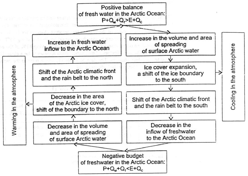
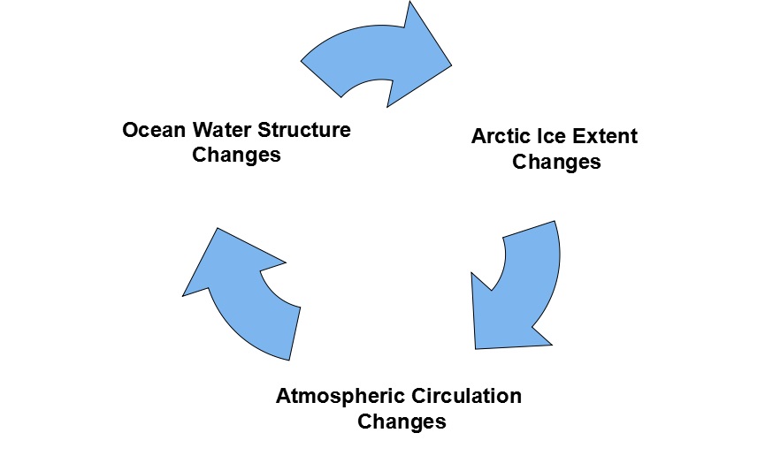
The really big paradigm shift is to understand that the sea ice extent itself regulates the periods of warming and cooling air temperatures, and not the other way around. Of course, there is a considerable lag, on the order of several decades, as you would expect in any system with massive capacity and momentum. Zakharov (here) shows how Arctic ice functions as a self-oscillating system:
Zacharov fig.24
Summary: Why the Arctic is not a Refrigerator
1. A fridge makes ice by keeping the air below freezing.
The Arctic makes ice by keeping warmer water away.
2. Ice melts in a fridge when warmer air is allowed in.
Ice melts in the Arctic when the sun shines.
3. The fridge is regulated by an air temperature sensor.
The Arctic is regulated by the ice extent itself.
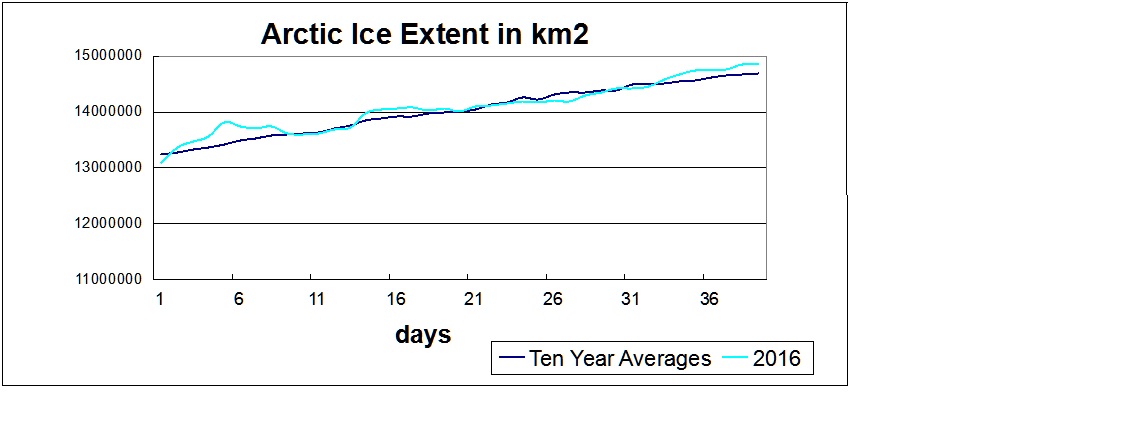
The media and warmists ignore Arctic ice in wintertime because they are obsessed with the summer melt, and hoping for lots of open water. In fact, ice extent trends are basically driven by the freezing this time of year, while Sept. extents vary greatly due to summer weather events, not climate change.
The press has been reporting some storm activity in the North Atlantic, and tossing words like “unprecedented” into the stories. But keeping things in perspective, we can say that the freezing is going normally with the usual day to day fluctuations.
January and February show an average year in progress:
Conclusion:
Do not trust mass media for unbiased reporting of climate news.
Some people don’t like the unalarming patterns of ice extents displayed by MASIE, and hang onto obsolete comments about times in the past when ice charts were inconsistent. Today’s MASIE dataset is accurate and reliable, according to NSIDC who expressed confidence when releasing it in 2015.
The NSIDC Sea Ice Index ice extent is widely used, but the edge position can be off by 10s or in some cases 100s of kilometers. NIC produces a better ice edge product, but it does not reach the same audience as the Sea Ice Index.
In June 2014, we decided to make the MASIE product available back to 2006. This was done in response to user requests, and because the IMS product output, upon which MASIE is based, appeared to be reasonably consistent. Note: Presently, NSIDC Sea Ice Index is showing ~700,000 km2 less ice extent than MASIE.
Post Paris sea level alarms are ramping up: As global temperatures rise, scientists know that sea levels will follow suit. Today, global sea level is the topic of two new papers, both published in Nature Climate Change. Source: Carbon Brief, today’s date.
Fortunately, antidotes for this feverish reporting are available. Some recent research reports published this year update our knowledge of sea ice and sea level dynamics. Two papers below are by Australians A.Parker and C. D. Ollier. They obviously are not employed by CSIRO, since they are working hard on understanding how the climate system actually works.
Is there a Quasi-60 years’ Oscillation of the Arctic Sea Ice Extent?
A.Parker and C. D. Ollier
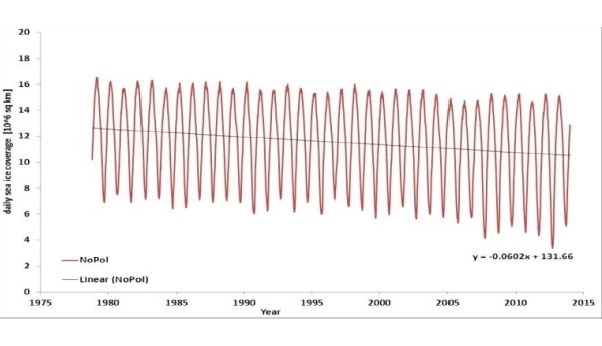
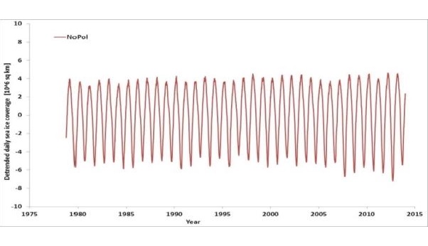
Satellite sea ice extent North Pole since 1979, the sea ice coverage anomalies. Data from NSIDC. The shrinking of ice is consistent with the warming temperature of Fig. 3.
From the Abstract: The Arctic sea ice experienced a drastic reduction that was phased with warming temperatures 1923 to 1940. This reduction was followed by a sharp cooling and sea ice recovery. This permits us to also conclude that very likely the Arctic sea ice extent also has a quasi-60 years’ oscillation. The recognition of a quasi-60 year’s oscillation in the sea ice extent of the Arctic similar to the oscillation of the temperatures and the other climate indices may permit us to separate the natural from the anthropogenic forcing of the Arctic sea ice. The heliosphere and the Earth’s magnetosphere may have much stronger influence on the climate patterns on Earth including the Arctic sea ices than has been thought.
Satellite sea ice extent North Pole since 1979, the values de-trended to the linear fitting line. Data are from NSIDC.
This finding is entirely consistent with Zakharov’s work at AARI, (here) and with analyses (here) of fluctuating Barents and Arctic Sea Ice.
Discussion of Foster & Brown’s Time and Tide: Analysis of Sea Level Time Series
A.Parker and C. D. Ollier
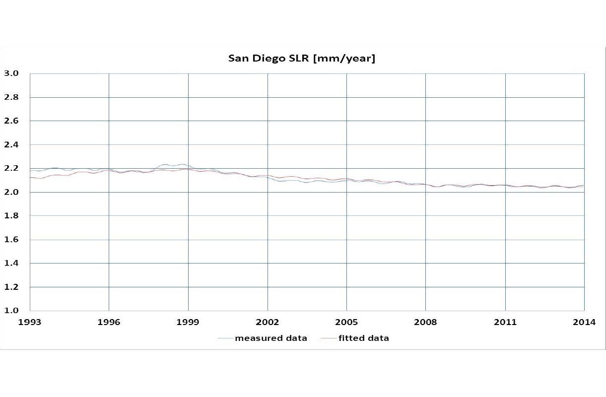
Sea level patterns in San Diego: SLR over the last 20 years.
From the Abstract: The recognition of the non-accelerating, periodic pattern of sea levels as described by the tide gauges measurements does not require any special mathematical tool. Providing enough data of sufficient quality have been recorded, If the classical linear fitting is used to compute the rate of rise at any time, then the acceleration is simply the time rate of change of this velocity. By using this technique, the lack of any acceleration over the last few decades is evident in the naturally oscillating, slow rising, tide gauges of appropriate quality and length.
If the sea levels have to rise 1 meter by 2100 and not only 21.5 millimeters at the worldwide average tide gauge, there is a problem of orders of magnitude difference in the sea levels computed (by climate models) and measured (by tide gauges). http://sciencedomain.org/abstract/8091
Postscript:
It has come to my attention that both Albert Parker and Cliff Ollier have been vilified on alarmist websites, and will likely be attacked again for their latest papers, which are continuing to favor observations over projections from climate models. For reference I provide additional responses from the two scientists to past critiques.
In a piece in the December 11 issue of NRC/Handelsblad, Rotterdam’s counterpart to the New York Times, Wilco Hazeleger, a senior scientist in the global climate research group at KNMI (the Royal Netherlands Meteorological Institute) wrote: “In the past century the sea level has risen twenty centimetres. There is no evidence for accelerated sea-level rise. It is my opinion that there is no need for drastic measures. … Fortunately, the time rate of climate change is slow compared to the life span of the defense structures along our coast. There is enough time for adaptation.”
It would be much better if our politicians (and some scientists) based their opinions on what we can actually observe about sea level, instead of alarming us with dreams of catastrophic sea level rise based on false models of what might be happening to ice caps. Of course even if we believed sea level is rising, it takes another leap of faith to think it is caused by miniscule increases in atmospheric carbon dioxide caused by human activity.
Parker replied to defenders of consensus climate science in 2013:
It is demonstrated that the IPCC models do not reproduce the natural harmonics as the quasi-60 years cycle and overestimate the effect of the anthropic forcings. The IPCC models are shown compatible with the 1999 Mann hockey stick but unfortunately for the IPCC also incompatible with the recent temperature reconstructions. The global warming and sea level predictions for the 21st century may be consequently equally wrong. The increased heat uptake or the rising temperatures of the oceans or the accelerating seas all have similar lack of sound scientific bases.
Yesterday I realized that BBC had blocked the viewing of the video. So I sought and found the subtitles for Yes Prime Minister 2013, Episode 6, “A Tsar is Born”. That final episode for the series began with the dialogue in yesterday’s post Climate Alarms LOL.
Today I provide the dialogue that formed the episode conclusion, and which was the content of the blocked video.
The Characters are:
Sir Humphrey Appleby
Cabinet Secretary
Jim Hacker
Prime Minister
Claire Sutton
Special Policy Adviser
Bernard Woolley
Principal Private Secretary to the Prime Minister
(Dialogue beginning at 20:16 of “A Tsar is Born”)
Humphrey I have returned with the answer to all your problems. Global warming.
Jim I thought you were against it?
Humphrey Everybody’s against it, Prime Minister. I suddenly realised that is the beauty of it. We can get a unanimous agreement with all of our European partners
to do something about it.
Jim But how can we do something about something that isn’t happening?
Humphrey It’s much easier to solve an imaginary problem than a real one.
Jim You believe it’s real?
Humphrey Do you? I don’t know.
Jim Neither do I. Haven’t got the faintest idea!
Humphrey But it doesn’t matter what we think. If everyone else thinks it’s real, they’ll all want to stop it. So long as it doesn’t cost too much. So the question now is, what are we going to do about it?
Jim But if it isn’t happening, what can we do about it?
Humphrey Oh, there’s so much we can do, Prime Minister. We can impose taxes, we can stiffen European rules about
carbon emissions, rubbish disposal. We can make massive investments in wind turbines. We can, in fact, Prime Minister, under your leadership, agree to save the world.
Jim Well, I like that! But Russia, India, China, Brazil, they’ll never cooperate.
Humphrey They don’t have to. We simply ask them to review their emissions policy.
Jim And will they?
Humphrey Yes. And then they’ll decide not to change it. So we’ll set up a series of international conferences. Meanwhile, Prime Minister, you can talk about the future of the planet.
Jim Yes.
Humphrey You can look statesmanlike. And it’ll be 50 years before anybody can possibly prove you’re wrong. And you can explain away anything you said before by saying the computer models were flawed.
Jim The voters will love me!
Humphrey You’ll have more government expenditure.
Jim Yes. How will we pay for it? We’re broke.
Humphrey We impose a special global warming tax on fuel now, but we phase in the actual expenditure gradually. Say, over 50 years? That will get us out of the hole for now.
Bernard The Germans will be pleased. They have a big green movement.
Claire And we can even get the progs on board!
Bernard As long as they get more benefits than everyone else.
Jim My broadcast is on Sunday morning.
Humphrey You have a day to get the conference to agree.
Jim That’s not a problem. The delegates will be desperate for something to announce when they get home. There is one problem. Nothing will have actually been achieved.
Humphrey It will sound as though it has. So people will think it has. That’s all that matters!
(Later following the BBC interview, beginning 27:34)
Bernard Oh, magnificent, Prime Minister!
Humphrey I think you got away with it, Jim, but the cabinet will have been pretty surprised. We’ll have to square them fast.
Jim Bubbles!
Humphrey We’re not there yet. After that interview, you’ll need to announce some pretty impressive action.
Jim An initiative.
Humphrey Yes.
Claire A working party?
Humphrey Bit lightweight.
Bernard A taskforce?
Humphrey Not sure.
Jim Do we have enough in the kitty?
Claire It could be one of those initiatives that you announce but never actually spend the money.
Jim Great. Like the one on child poverty.
Bernard Maybe it should be a government committee?
Jim Well what about a Royal Commission?
Humphrey Yes! It won’t report for three years, and if we put the right people on it, they’ll never agree about anything important.
Jim Right! A Royal Commission! No, wait a minute, that makes it sound as if we think it’s important but not urgent.
Claire Well, what about a Global Warming Tsar?
Jim Fine! Would that do it?
Humphrey No, I think it might need a bit more than that, Prime Minister. It’ll mean announcing quite a big unit, and an impressive salary for that Tsar, to show how much importance you place upon him.
Jim No problem. Who would it be?
Humphrey Ah, well, it can’t be a political figure. That would be too divisive. It has to be somebody impartial.
Jim You mean a judge?
Humphrey No, somebody from the real world. Somebody who knows how to operate the levers of power, to engage the gears of the Whitehall machine, to drive the engine of government.
Jim That’s quite a tall order. Anybody got any ideas?
Humphrey… Could you?
Bernard Oh!
Humphrey Yes, Prime Minister.
The End.
Footnote
CO2 hysteria is addictive. Here’s what it does to your brain:
His main point from the abstract: The marine environment of North Sea and Baltic is one of the most heavily strained by numerous human activities. Simultaneously water and air temperatures increase more than elsewhere in Europe and globally, which cannot be explained with “global warming”.
Excerpts:
Since mankind, during the course of a year, agitates the water column of North Sea and Baltic by stirring, more warmth is taken to deeper water in the summer season and rises to the surface from lower layers in the winter period, where heat is exchanged with the air until sea icing is observed. This is a process that can be seen from the beginning of September until the end of March.
Marine activities play a much bigger role in time factor and duration of ice formation. If the sea surface temperature has already reached the freezing point, any vessel shovels warmer water to the surface, or vice versa, forcing a more rapid melt… The shrinking ice cover correlates well with an increase in human activities, and subsequently leading to higher air temperature throughout the region.
Basically three facts are established: higher warming, a small shift in the seasons, and a decreasing sea ice cover. In each scenario the two seas’ conditions play a decisive role (North Sea and Baltic). These conditions are impaired by wind farms, shipping, fishing, off shore drilling, under sea floor gas-pipe line construction and maintenance, naval exercise, diving, yachting, and so on, about little to nothing has been investigated and is understood.
Summary The facts are conclusive. “Global Climate Change” cannot cause a special rise in temperatures in Northern Europe, neither in the North Sea nor the Baltic or beyond. Any use of the oceans by mankind has an influence on thermo-haline structures within the water column from a few cm to 10m and more. Noticeable warmer winters in Europe are the logical consequence.
North Americans should not think themselves unaffected by all this.
Consider this graphic of the Siberian Express:
The more the Atlantic weather governs the situation beyond the Ural the further Polar and Siberian cold will be pushed eastwards, called ‘Siberian Express’(Fig.10). This was felt in Alaska, Canada and Eastern U.S. Many days were extremely cold with deviations from the mean of 20°C and beyond.
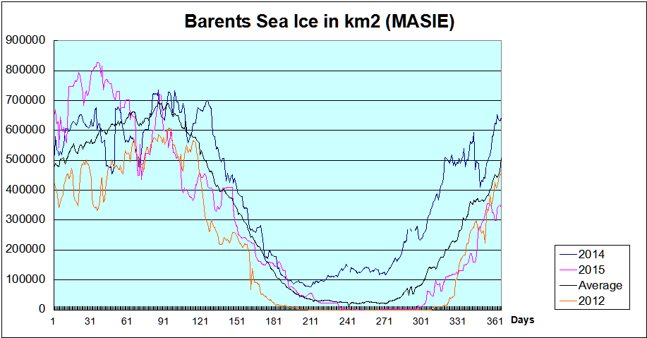
A chart of Barents Ice Cycles looks a lot like the icicles above, except upside down since Barents Sea is usually all water by September. Notice the black lines in the graph below hitting bottom near zero.
Note also the anomalies in red are flat until 1998, then decline to 2007 and then flat again.
Why Barents Sea Ice Matters
Barents Sea is No. 1, being located at the gateway between the Arctic and North Atlantic. Previous posts (here and here) have discussed research suggesting that changes in Barents Sea Ice may signal changes in Arctic Sea Ice a few years later. As well, the studies point to changes in heat transport from the North Atlantic driving the Barents Sea Ice, along with changes in salinity of the upper layer. And, as suggested by Zakharov (here), there are associated changes in atmospheric circulations, such as the NAO (North Atlantic Oscillation).
Here we look at MASIE over the last decade and other datasets over longer terms in search for such patterns.
Observed Barents Sea Ice
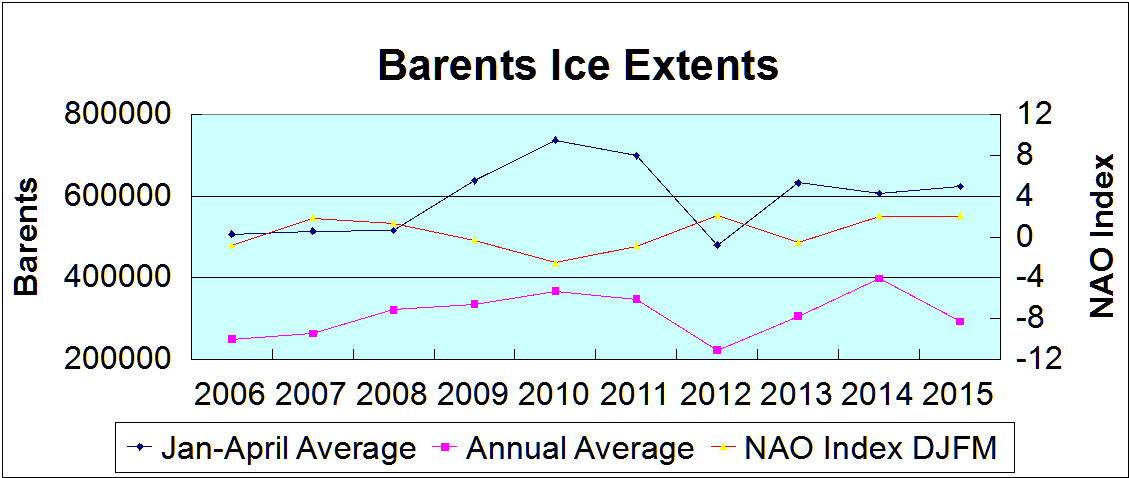
Below is a more detailed look at recent years.
This graph shows that the last two years were outliers in opposite directions. 2014 was an exceptionally high annual average due to melting delayed until April, and then a much higher minimum and faster than average recovery. In contrast 2015 was high initially, became average by day 91, then dropped sharply to a meltout, followed by a slower recovery. 2012 shows the lowest Barents ice year contrasting with 2014, the highest annual extent in the last decade.
Annual average BSIE (Barents Sea Ice Extent) is 315k km2, varying between 250k and 400k over the last ten years. The volatility is impressive, considering the daily Maximums and Minimums in the record. Average Max is 781k, ranging from 608k to 936k. Max occurs on day 77 (average) with a range from day 36 to 103. Average Min is 11k on day 244, ranging from 0k to 77k, and from days 210 to 278.
In fact, over this decade, there are not many average years. Five times BSIE melted to zero, two were about average, and 3 years much higher: 2006-7 were 2 and 3 times average, and 2014 was 7 times higher at 77k.
As for Maxes, only 1 year matched the 781k average. Four low years peaked at about 740k (2006,07,08 and 14), and the lowest year at 608k (2012). The four higher years start with the highest one, 936k in 2010, and include 2011, 13, and 15.
Comparing Barents Ice and NAO
This graph confirms that Barents winter extents (JFMA) correlate strongly (0.73) with annual Barents extents. And there is a slightly less strong inverse correlation with NAO index (-0.64). That means winter NAO in its negative phase is associated with larger ice extents, and vice-versa.
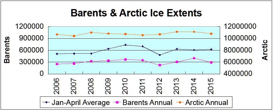
Comparing Barents Ice and Arctic Annual
Arctic Annual extents correlate with Barents Annuals at a moderately strong 0.46, but have only weaker associations with winter NAO or Barents winter averages. It appears that 2012 and 2015 interrupted a pattern of slowly rising extents.
NAO and Arctic Ice Longer Term
Fortunately there are sources providing an history of Arctic ice longer term and overlapping with the satellite era. For example:
Mahoney et al say this about Arctic Ice oscillations:
We can therefore broadly divide the ice chart record into three periods. Period A, extending from the beginning of the record until the mid-1950s, was a period of declining summer sea ice extent over the whole Russian Arctic, though not consistently in every individual sea. . . Period B extended from the mid-1950s to the mid- 1980s and was a period of generally increasing or stable summer sea ice extent. For the Russian Arctic as a whole, this constituted a partial recovery of the sea ice lost during period A, though this is not the case in all seas. . . Period C began in the mid-1980s and continued to the end of the record (2006). It is characterized by a decrease in total and MY sea ice extent in all seas and seasons.
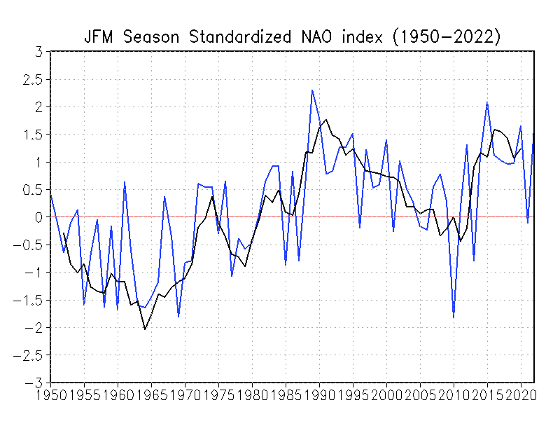
Comparing Arctic Ice with winter NAO index
The standardized seasonal mean NAO index during cold season (blue line) is constructed by averaging the monthly NAO index for January, February and March for each year. The black line denotes the standardized five-year running mean of the index. Both curves are standardized using 1950-2000 base period statistics.
The graph shows roughly a 60 year cycle, with a negative phase 1950-1980 and positive 1980 to 2010. As described above, Arctic ice extent grew up to 1979, the year satellite ice sensing started, and declined until 2007. The surprising NAO uptick recently coincides with the anomalous 2012 and 2015 meltings.
As of January 2016 NAO has gone negative for the first time in months.
Summary
If the Barents ice cycle repeats itself over the next decades, we should expect Arctic ice extents to grow as part of a natural oscillation. The NAO atmospheric circulation pattern is part of an ocean-ice-atmosphere system which is driven primarily by winter changes in the North Atlantic upper water layer.
The original post and updates were done in October 2015. Now Radford Neal has done a complete deconstruction of the published paper in his post (here): Critique of ‘Debunking the climate hiatus’, by Rajaratnam, Romano, Tsiang, and Diffenbaugh . Neal says:
Climatic Change appears to be a reputable refereed journal, which is published by Springer, and which is cited in the latest IPCC report. The paper was touted in popular accounts as showing that the whole hiatus thing was mistaken — for instance, by Stanford University itself.
You might therefore be surprised that, as I will discuss below, this paper is completely wrong. Nothing in it is correct. It fails in every imaginable respect.
Original post and updates October 3 and 30 below
With Paris COP drawing near, the lack of warming this century is inconvenient and undermines the cause.
As Dr. Judith Curry said, “I have been expecting to start seeing papers on the ‘hiatus is over.’ Instead I am seeing papers on ‘the hiatus never happened.’”
One that was trumpeted came out of my Alma Mater, Stanford. They garnered the expected headlines from the usual places:
Global Warming “Hiatus” Never Happened: Eos
There never was any global warming “pause.”: Washington Post
We don’t need to get into the technicalities of why they stopped with 2013 data, the suitability of the tests applied or their interpretations of the results.
Here’s what you need to know about this study:
They ignored the satellite records (RSS and UAH), the gold standard of temperature measurements, because the absence of warming there is undeniable.
For the land and ocean datasets they analyzed, they ignored the huge divergence between observations and the predictions (projections) from climate models.
Conclusion:
Natural variability in the climate system has neutralized any warming from increased CO2 this century, and also offset most, if not all of the secular rise in temperature since the Little Ice Age. The models did not forecast this; they can only project warming, and do so at rates several times higher than observations. The models fail for three reasons: high sensitivity to CO2; positive feedback from water vapor; and lack of thermal inertia by the oceans.
The Stanford football team was impressive beating highly-rated Southern Cal on their home field last Saturday. The work of the research team, however, looks like pandering rather than science. They need to up their game: No cookies.
Update October 3
I found the time to look into the details of this paper and the statistical trick comes to light.
They took as the null hypothesis: “Temperatures are not rising.” After applying several statistical tests, they conclude that the statement is not supported by the data, so we cannot say with certainty temperatures are not rising.
And what about the other null hypothesis: “Temperatures are rising.” Silence.
I suspect they didn’t want to admit that the same statistical tests would also disprove that statement.
A reasonable person concludes: When you can not say for sure that temperatures are not rising, or that they are rising, that would surely indicate a plateau in temperatures.