Greenhouse with adjustable sun screens to control warming.
Update July 12, 2019
A paper was just published by an IPCC reviewer No Empirical Evidence for Significant Anthropogenic Climate Change by J. Kauppinen and P. Malmi. Excerpts in italics with my bolds. H/T WUWT
An analysis by Finnish researchers adds to the chain of studies supporting the Cosmoclimatology theory first proposed by Svensmark. Their focus is on the relation between the changes in temperatures and the changes in low cloud cover. Their findings are consistent with the global brightening and dimming research centered at ETH Zurich, which is elaborated later on.

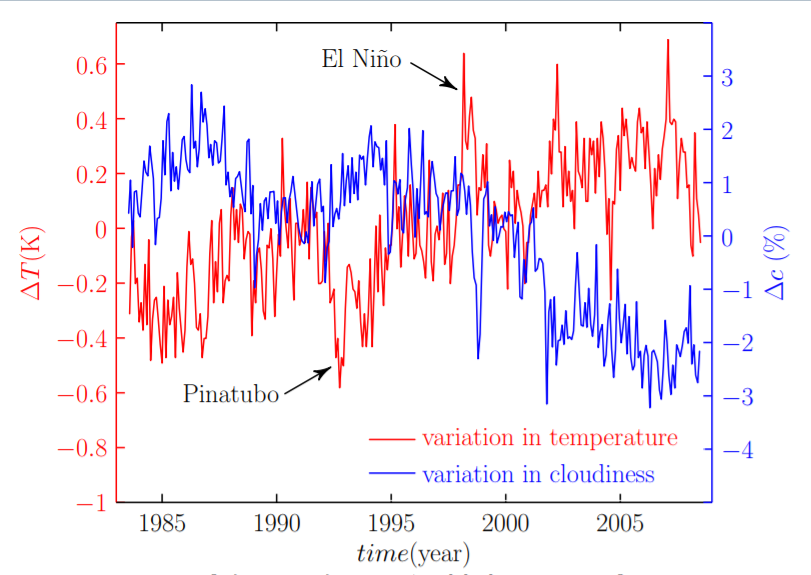
Figure 2. [2] Global temperature anomaly (red) and the global low cloud cover changes (blue) according to the observations. The anomalies are between summer 1983 and summer 2008. The time resolution of the data is one month, but the seasonal signal is removed. Zero corresponds about 15°C for the temperature and 26 % for the low cloud cover.
It turns out that the
changes in the relative humidity and in the low cloud cover depend on each other [4]. So, instead of low cloud cover we can use the changes of the relative humidity in order to derive the natural temperature anomaly.
According to the observations 1 % increase of the relative humidity decreases the temperature by 0.15°C, and consequently the last term in the above equation can be approximated by −15°C∆φ, where ∆φ is the change of the relative humidity at the altitude of the low clouds.
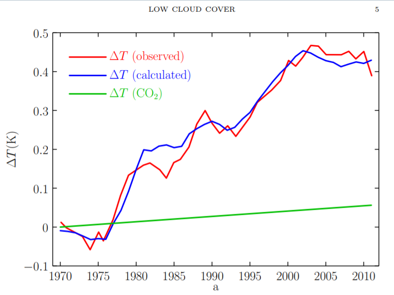
Figure 4 shows the sum of the temperature changes due to the natural and CO2 contributions compared with the observed temperature anomaly. The natural component has been calculated using the changes of the relative humidity. Now we see that the natural forcing does not explain fully the observed temperature anomaly. So we have to
add the contribution of CO2 (green line), because the time interval is now 40 years (1970–2010). The concentration of CO2 has now increased from 326 ppm to 389 ppm. The green line has been calculated using the sensitivity 0.24°C, which seems to be correct. In Fig. 4 we see clearly how well a change in the relative humidity can model the strong temperature minimum around the year 1975. This is impossible to interpret by CO2 concentration.
 The IPCC climate sensitivity is about one order of magnitude too high, because a strong negative feedback of the clouds is missing in climate models. If we pay attention to the fact that only a small part of the increased CO2 concentration is anthropogenic, we have to recognize that the anthropogenic climate change does not exist in practice. The major part of the extra CO2 is emitted from oceans [6], according to Henry‘s law. The low clouds practically control the global average temperature. During the last hundred years the temperature is increased about 0.1°C because of CO2. The human contribution was about 0.01°C.
We have proven that the GCM-models used in IPCC report AR5 cannot compute correctly the natural component included in the observed global temperature. The reason is that the models fail to derive the influences of low cloud cover fraction on the global temperature. A too small natural component results in a too large portion for the contribution of the greenhouse gases like carbon dioxide. That is why IPCC represents the climate sensitivity more than one order of magnitude larger than our sensitivity 0.24°C. Because the anthropogenic portion in the increased CO2 is less than 10 %, we have practically no anthropogenic climate change. The low clouds control mainly the global temperature.
Previous Update Hard Evidence of Solar Impact upon Earth Cloudiness
Later on is a reprinted discussion of global dimming and brightness resulting from fluctuating cloud cover. This is topical because of new empirical research findings coming out of Asia. H/T GWPF. A study published by Kobe University research center is Revealing the impact of cosmic rays on the Earth’s climate. Excerpts in italics with my bolds.

New evidence suggests that high-energy particles from space known as galactic cosmic rays affect the Earth’s climate by increasing cloud cover, causing an “umbrella effect”.
When galactic cosmic rays increased during the Earth’s last geomagnetic reversal transition 780,000 years ago, the umbrella effect of low-cloud cover led to high atmospheric pressure in Siberia, causing the East Asian winter monsoon to become stronger. This is evidence that galactic cosmic rays influence changes in the Earth’s climate. The findings were made by a research team led by Professor Masayuki Hyodo (Research Center for Inland Seas, Kobe University) and published on June 28 in the online edition of Scientific Reports.
The Svensmark Effect is a hypothesis that galactic cosmic rays induce low cloud formation and influence the Earth’s climate. Tests based on recent meteorological observation data only show minute changes in the amounts of galactic cosmic rays and cloud cover, making it hard to prove this theory. However, during the last geomagnetic reversal transition, when the amount of galactic cosmic rays increased dramatically, there was also a large increase in cloud cover, so it should be possible to detect the impact of cosmic rays on climate at a higher sensitivity.

(The Svensmark Effect is explained in essay The cosmoclimatology theory)
How Nature’s Sunscreen Works (from Previous Post)
A recent post Planetary Warming: Back to Basics discussed a recent paper by Nikolov and Zeller on the atmospheric thermal effect measured on various planets in our solar system. They mentioned that an important source of temperature variation around the earth’s energy balance state can be traced to global brightening and dimming.
This post explores the fact of fluctuations in the amount of solar energy reflected rather than absorbed by the atmosphere and surface. Brightening refers to more incoming solar energy from clear and clean skies. Dimming refers to less solar energy due to more sunlight reflected in the atmosphere by the presence of clouds and aerosols (air-born particles like dust and smoke).
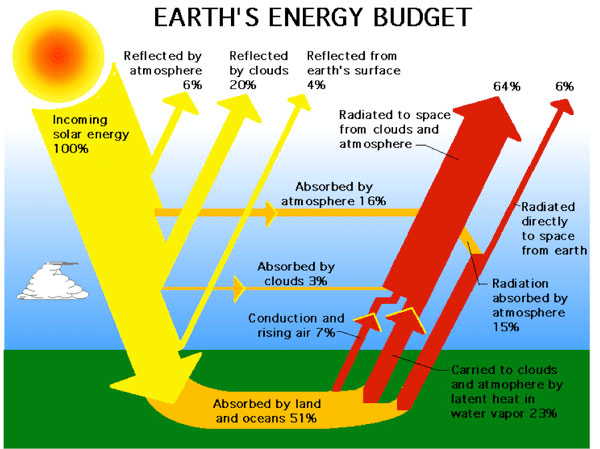
The energy budget above from ERBE shows how important is this issue. On average, half of sunlight is either absorbed in the atmosphere or reflected before it can be absorbed by the surface land and ocean. Any shift in the reflectivity (albedo) impacts greatly on the solar energy warming the planet.
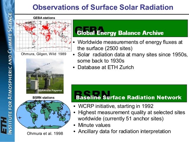
The leading research on global brightening/dimming is done at the Institute for Atmospheric and Climate Science of ETH Zurich, led by Martin Wild, senior scientist specializing in the subject.
Special instruments have been recording the solar radiation that reaches the Earth’s surface since 1923. However, it wasn’t until the International Geophysical Year in 1957/58 that a global measurement network began to take shape. The data thus obtained reveal that the energy provided by the sun at the Earth’s surface has undergone considerable variations over the past decades, with associated impacts on climate.
The initial studies were published in the late 1980s and early 1990s for specific regions of the Earth. In 1998 the first global study was conducted for larger areas, like the continents Africa, Asia, North America and Europe for instance.
Now ETH has announced The Global Energy Balance Archive (GEBA) version 2017: A database for worldwide measured surface energy fluxes. The title is a link to that paper published in May 2017 explaining the facility and some principal findings. The Archive itself is at http://www.geba.ethz.ch.
For example, Figure 2 below provides the longest continuous record available in GEBA: surface downward shortwave radiation measured in Stockholm since 1922. Five year moving average in blue, 4th order regression model in red. Units Wm-2. Substantial multidecadal variations become evident, with an increase up to the 1950s (“early brightening”), an overall decline from the 1950s to the 1980s (“dimming”), and a recovery thereafter (“brightening”).
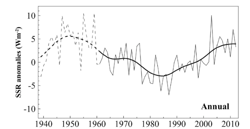
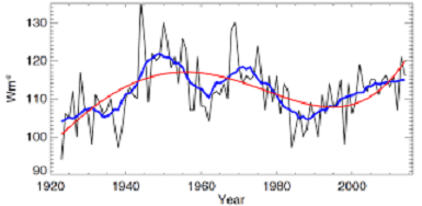 Figure 5. Composite of 56 European GEBA time series of annual surface downward shortwave radiation (thin line) from 1939 to 2013, plotted together with a 21 year Gaussian low-pass filter ((thick line). The series are expressed as anomalies (in Wm-2) from the 1971–2000 mean. Dashed lines are used prior to 1961 due to the lower number of records for this initial period. Updated from Sanchez-Lorenzo et al. (2015) including data until December 2013.
 Martin Wild explains in a 2016 article Decadal changes in radiative fluxes at land and ocean surfaces and their relevance for global warming. From the Conclusion (SSR refers to solar radiation incident upon the surface)
However, observations indicate not only changes in the downward thermal fluxes, but even more so in their solar counterparts, whose records have a much wider spatial and temporal coverage. These records suggest multidecadal variations in SSR at widespread land-based observation sites. Specifically, declining tendencies in SSR between the 1950s and 1980s have been found at most of the measurement sites (‘dimming’), with a partial recovery at many of the sites thereafter (‘brightening’).

With the additional information from more widely measured meteorological quantities which can serve as proxies for SSR (primarily sunshine duration and DTR), more evidence for a widespread extent of these variations has been provided, as well as additional indications for an overall increasing tendency in SSR in the first part of the 20th century (‘early brightening’).
It is well established that these SSR variations are not caused by variations in the output of the sun itself, but rather by variations in the transparency of the atmosphere for solar radiation. It is still debated, however, to what extent the two major modulators of the atmospheric transparency, i.e., aerosol and clouds, contribute to the SSR variations.

The balance of evidence suggests that on longer (multidecadal) timescales aerosol changes dominate, whereas on shorter (decadal to subdecadal) timescales cloud effects dominate. More evidence is further provided for an increasing influence of aerosols during the course of the 20th century. However, aerosol and clouds may also interact, and these interactions were hypothesized to have the potential to amplify and dampen SSR trends in pristine and polluted areas, respectively.
No direct observational records are available over ocean surfaces. Nevertheless, based on the presented conceptual ideas of SSR trends amplified by aerosol–cloud interactions over the pristine oceans, modeling approaches as well as the available satellite-derived records it appears plausible that also over oceans significant decadal changes in SSR occur.
The coinciding multidecadal variations in SSTs and global aerosol emissions may be seen as a smoking gun, yet it is currently an open debate to what extent these SST variations are forced by aerosol-induced changes in SSR, effectively amplified by aerosol– cloud interactions, or are merely a result of unforced natural variations in the coupled ocean atmosphere system. Resolving this question could state a major step toward a better understanding of multidecadal climate change.

Another paper co-authored by Wild discusses the effects of aerosols and clouds The solar dimming/brightening effect over the Mediterranean Basin in the period 1979 − 2012. (NSWR is Net Short Wave Radiation, that is equal to surface solar radiation less reflected)
The analysis reveals an overall increasing trend in NSWR (all skies) corresponding to a slight solar brightening over the region (+0.36 Wm−2per decade), which is not statistically significant at 95% confidence level (C.L.). An increasing trend(+0.52 Wm−2per decade) is also shown for NSWR under clean skies (without aerosols), which is statistically significant (P=0.04).
This indicates that NSWR increases at a higher rate over the Mediterranean due to cloud variations only, because of a declining trend in COD (Cloud Optical Depth). The peaks in NSWR (all skies) in certain years (e.g., 2000) are attributed to a significant decrease in COD (see Figs. 9 and 10), whilethe two data series (NSWRall and NSWRclean) are highly correlated(r=0.95).
This indicates that cloud variation is the major regulatory factor for the amount and multi-decadal trends in NSWR over the Mediterranean Basin. (Note: Lower cloud optical depth is caused by less opaque clouds and/or decrease in overall cloudiness)
On the other hand, the results do not reveal a reversal from dimming to brightening during 1980s, as shown in several studies over Europe (Norris and Wild, 2007;Sanchez-Lorenzoet al., 2015), but a rather steady slight increasing trend in solar radiation, which, however, seems to be stabilized during the last years of the data series, in agreement with Sanchez-Lorenzo et al. (2015). Similarly, Wild (2012) reported that the solar brightening was less distinct at European sites after 2000 compared to the 1990s.
In contrast, the NSWR under clear (cloudless) skies shows a slight but statistically significant decreasing trend (−0.17 Wm−2per decade,P=0.002), indicating an overall decrease in NSWR over the Mediterranean due to water-vapor variability suggesting a transition to more humid environment under a warming climate.

Other researchers find cloudiness more dominant than aerosols. For example, The cause of solar dimming and brightening at the Earth’s surface during the last half century: Evidence from measurements of sunshine duration by Gerald Stanhill et al.
Analysis of the Angstrom-Prescott relationship between normalized values of global radiation and sunshine duration measured during the last 50 years made at five sites with a wide range of climate and aerosol emissions showed few significant differences in atmospheric transmissivity under clear or cloud-covered skies between years when global dimming occurred and years when global brightening was measured, nor in most cases were there any significant changes in the parameters or in their relationships to annual rates of fossil fuel combustion in the surrounding 1° cells. It is concluded that at the sites studied changes in cloud cover rather than anthropogenic aerosols emissions played the major role in determining solar dimming and brightening during the last half century and that there are reasons to suppose that these findings may have wider relevance.
Summary
The final words go to Martin Wild from Enlightening Global Dimming and Brightening.
Observed Tendencies in surface solar radiation
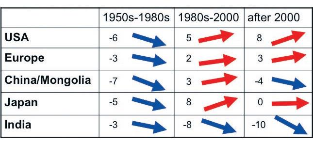
 Figure 2. Changes in surface solar radiation observed in regions with good station coverage during three periods.(left column) The 1950s–1980s show predominant declines (“dimming”), (middle column) the 1980s–2000 indicate partial recoveries (“brightening”) at many locations, except India, and (right column) recent developments after 2000 show mixed tendencies. Numbers denote typical literature estimates for the specified region and period in W m–2 per decade. Based on various sources as referenced in Wild (2009).
The latest updates on solar radiation changes observed since the new millennium show no globally coherent trends anymore (see above and Fig. 2). While brightening persists to some extent in Europe and the United States, there are indications for a renewed dimming in China associated with the tremendous emission increases there after 2000, as well as unabated dimming in India (Streets et al. 2009; Wild et al. 2009).
We cannot exclude the possibility that we are currently again in a transition phase and may return to a renewed overall dimming for some years to come.
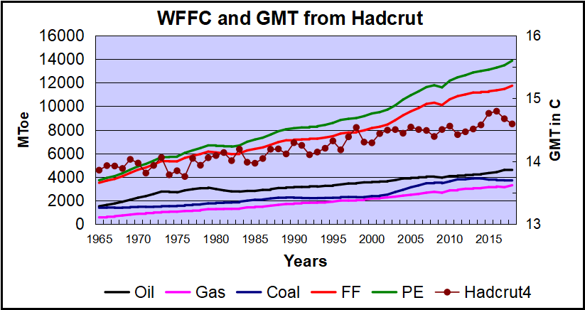
One can’t help but see the similarity between dimming/brightening and patterns of Global Mean Temperature, such as HadCrut.

Footnote: For more on clouds, precipitation and the ocean, see Here Comes the Rain Again

 Joel Kotkin makes sense of the confusing US politics around the 2020 presidential campaigning. He writes A class guide to the 2020 presidential election in Orange County Register. Excerpts in italics with my bolds.


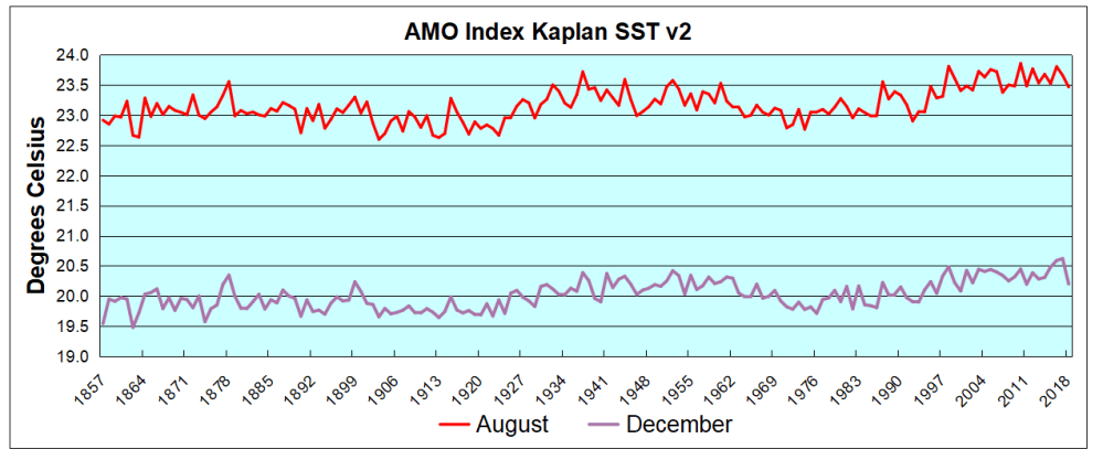
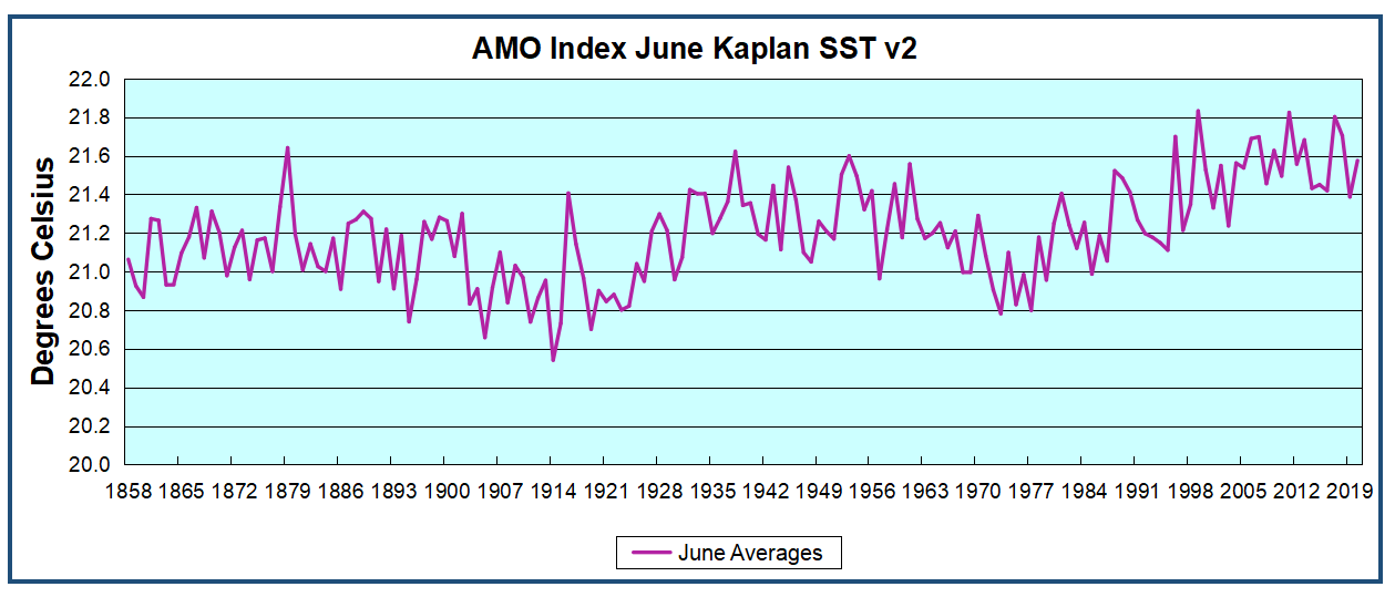
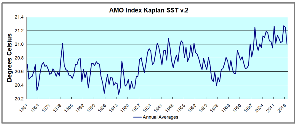
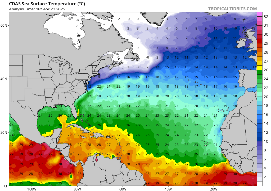
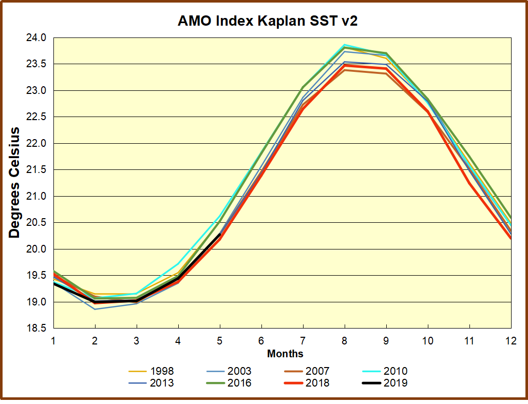
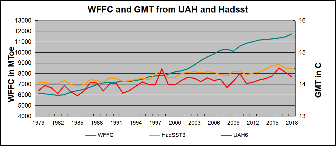
 The best context for understanding decadal temperature changes comes from the world’s sea surface temperatures (SST), for several reasons:
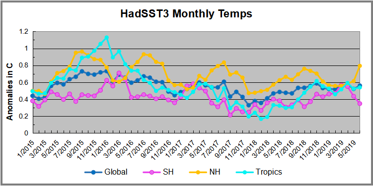
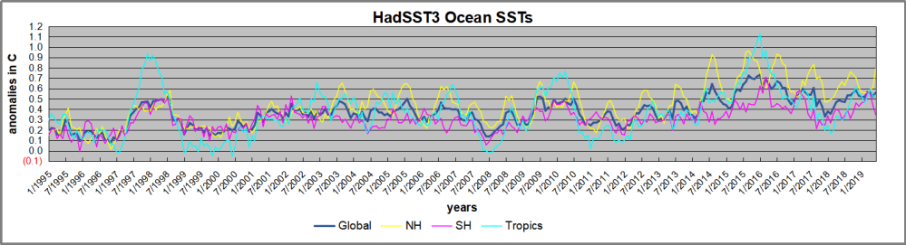 Open image in new tab to enlarge.
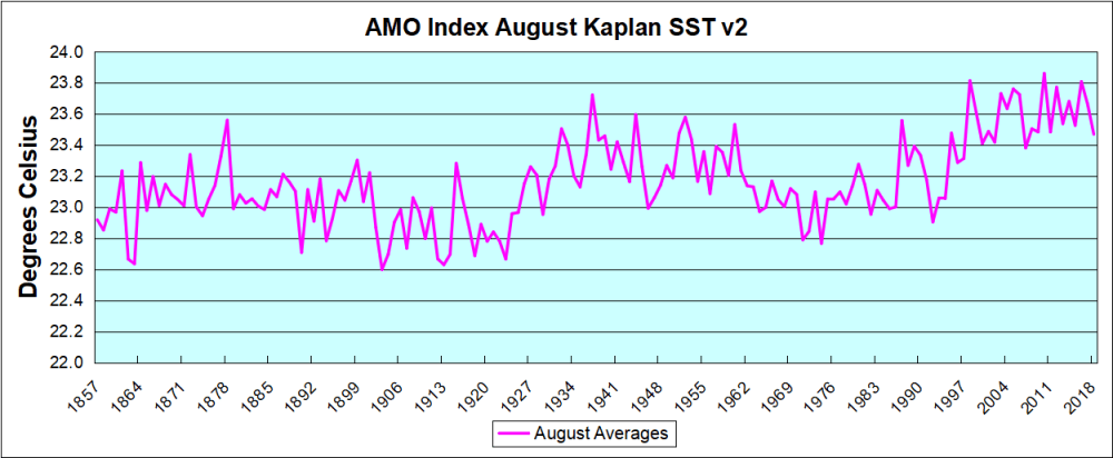

 The image above is from the Hunt for Red October (1990). Sean Connery played Marko Alexandrovich Ramius, a Soviet submarine captain, here in a confrontation with the on board Political Officer Ivan Putin, responsible to ensure the crew conforms to the Communist Party Line and Directives.


/null-hypothesis-examples-609097_FINAL-100262e70b70426fb0633304eb2f49f4.png)


 See Also