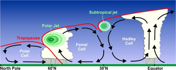
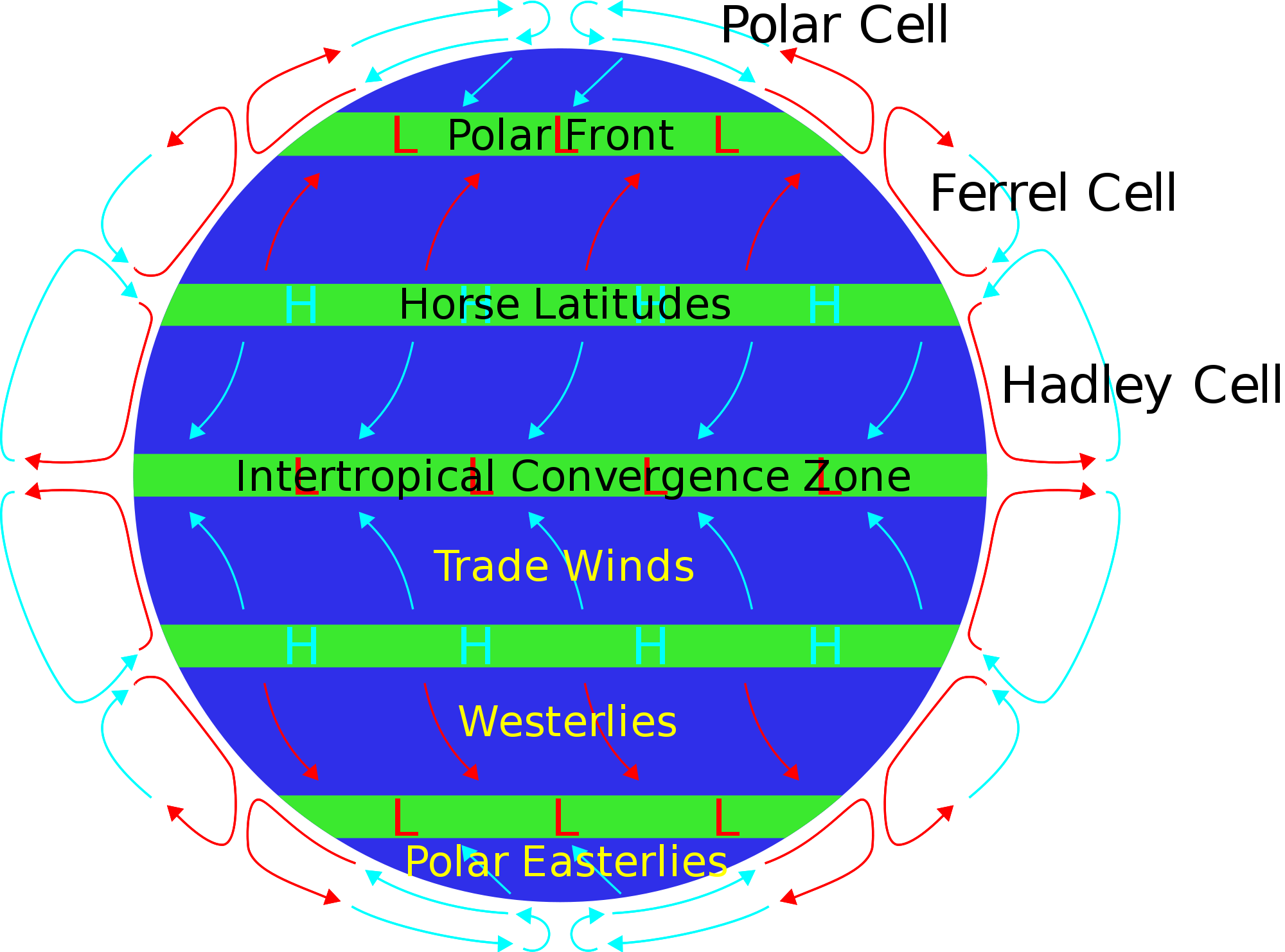
The subtropical jet streams are weaker and higher in the atmosphere at 10-16 kilometers above sea level. Jet streams wander laterally in quite dramatic waves and can exhibit huge changes in altitude. Breaks in the tropopause at the Polar, Hadley and Ferrel circulation cells cause the streams to form. The combination of circulation and Coriolis forces acting on the cell masses drive the phenomenon. The Polar jet, being at a lower altitude, strongly affects weather and aviation. It is most often found between the latitudes of 30 degrees and 60 degrees, while you can find the subtropical jets at 30 degrees. A jet stream is generally a few hundred kilometers wide and only about 5 kilometers high.
Fundamental questions and unknowns concerning natural climate change are presented in this 2007 essay Challenges to Our Understanding of the General Circulation: Abrupt Climate Change by Richard Seager and David S. Battisti. Excerpts in italics with my bolds.
The abrupt climate changes that occurred during the last glaciation and deglaciation are mind boggling both in terms of rapidity and magnitude. That winters in the British Isles could switch between mild, wet ones very similar to today and ones in which winter temperatures dropped to as much as 20◦C below freezing, and do so in years to decades, is simply astounding. No state-of-the-art climate model, of the kind used to project future climate change within the Intergovernmental Panel on Climate Change process, has ever produced a climate change like this.
The problem for dynamicists working in this area is that the period of instrumental observations, and model simulations of that period, do not provide even a hint that drastic climate reorganizations can occur. Our understanding of the general circulation is based fundamentally on this period or, more correctly, on the last 50 years of it, a time of gradual climate change or, at best, more rapid changes of modest amplitude. So it is not surprising that our encyclopedia of knowledge of the general circulations contains many ideas of negative feedbacks between circulation features that may help explain climate variability but also stabilize the climate (Bjerknes 1964; Hazeleger et al. 2005; Shaffrey and Sutton 2004). The modern period has not been propitious for studying how the climate can run away to a new state. Because of this, our understanding has to be limited
The normal explanation of how such changes occurred is that deepwater formation in the Nordic Seas abruptly ceased or resumed forcing a change in ocean heat flux convergence and changes in sea ice. However, coupled GCMs only produce such rapid cessations in response to unrealistically large freshwater forcing and have not so far produced a rapid resumption.
The discussions of the spatial extent of abrupt climate changes in glacial times and during the last deglaciation should make it clear that the causes must be found in changes in the general circulations of the global, as opposed to regional, atmosphere and ocean circulation. The idea that the THC changes and directly impacts a small area of the globe, and that somehow most of the rest of the world piggy-backs along in a rather systematic and reliable way seems dubious.
Thus the problems posed by abrupt change in the North Atlantic region are:
1. How could sea ice extend so far south in winter during the stadials?
2. How, during the spring and summer of stadials, can there be such an enormous influx of heat as to melt the ice and warm the water below by close to 10◦C? If 50 m of water needs to be warmed up by this much in four months, it would take an average net surface heat flux of 150 Wm−2, more than twice the current average between early spring and midsummer and more than can be accounted for by any increase in summer solar irradiance (as during the Younger Dryas).
3. How can this stadial state of drastic seasonality abruptly shift into one similar to that of today with a highly maritime climate in western Europe? Remember that both states can exist in the presence of large ice sheets over North America and Scandinavia.
In thinking of ways to reduce the winter convergence of heat into the mid and high-latitude North Atlantic, we might begin with the storm tracks and mean atmosphere circulation. The Atlantic storm track and jet stream have a clear southwest-to-northeast trajectory, whereas the Pacific ones are more zonal over most of their longitudinal reach (Hoskins and Valdes 1990). If the Atlantic storm track and jet could be induced to take a more zonal track, akin to its Pacific cousin, the North Atlantic would cool.
Here we have argued that the abrupt changes must involve more than changes in the North Atlantic Ocean circulation. In particular it is argued that the degree of winter cooling around the North Atlantic must be caused by a substantial change in the atmospheric circulation involving a great reduction of atmospheric heat transport into the region. Such a change could, possibly, be due to a switch to a regime of nearly zonal wind flow across the Atlantic, denying western Europe the warm advection within stationary waves that is the fundamental reason for why Europe’s winters are currently so mild. Such a change in wind regime would, presumably, also cause a change in the North Atlantic Ocean circulation as the poleward flow of warm, salty waters from the tropics into the Nordic Seas is diverted south by the change in wind stress curl. This would impact the location and strength of deep water formation and allow sea ice to expand south.

The North Atlantic Oscillation (NAO) is is a largely atmospheric mode from fluctuations in the difference of atmospheric pressure at sea level (SLP) between the Icelandic low and the Azores high. Through fluctuations in the strength of the Icelandic low and the Azores high, it controls the strength and direction of westerly winds and location of storm tracks across the North Atlantic. It is part of the Arctic oscillation, and varies over time with no particular periodicity. Wikipedia
Recent Wind Research
A decade later we have further insight into the role of winds in climate change by means of a paper discussed in this Futurity article Wind shifts may explain Europe’s ‘weird’ winters Excerpts in italics with my bolds.
In the mid-1990s, scientists assembled the first century-long record of North Atlantic sea surface temperatures and quickly discovered a cycle of heating and cooling at the surface of the ocean. Each of these phases lasted for decades, even as temperatures warmed overall during the course of the century. Since this discovery, these fluctuations in ocean temperature have been linked to all manner of Northern Hemisphere climate disturbances, from Sahel drought to North Atlantic hurricanes.
Research also linked European climate variability to the temperature swings of its neighboring ocean in the spring, summer, and fall. Surprisingly, however, no imprint of the ocean’s variability could be found in Western Europe’s wintertime temperature record. This absence was especially puzzling in light of the fact that Europe’s mild winters are a direct consequence of its enviable location downwind of the North Atlantic.
Now, a study by researchers at McGill University and the University of Rhode Island suggests the answer to this puzzle lies in the winds themselves. The fluctuations in ocean temperature are accompanied by shifts in the winds. These wind shifts mean that air arrives in Western Europe via very different pathways in decades when the surface of the North Atlantic is warm, compared to decades when it is cool.
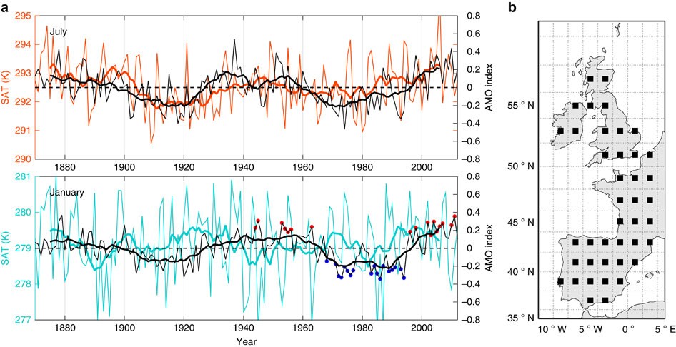
(a) Time series of the linearly detrended North Atlantic SST (black lines, referred to as the AMO index) and SAT averaged over western Europe ([36N 60N] × [10W 3E]; shown in coloured lines) in July (top panel) and January (bottom panel). Bold lines show 10-year running means. The correlation coefficient between the 10-year running mean of the detrended SAT and AMO index is 0.61 in July (statistically significant at 10% confidence level even after accounting for the reduced effective degrees of freedom due to autocorrelation of the time series) and −0.02 in January; these correlations are insensitive to the averaging region chosen for western Europe. The red circles on January plot indicate the AMO-positive years chosen for the composite analysis, whereas the blue circles indicate the AMO-negative years chosen. (b) Study region encompassing western Europe ([36N 60N] × [10W 3E]) and locations for the backtracked Lagrangian particle release (black squares).
The new research reveals that in decades in which North Atlantic sea surface temperatures are elevated, winds deliver air to Europe disproportionately from the north.
In contrast, in decades of coolest sea surface temperature, swifter winds extract more heat from the western and central Atlantic before arriving in Europe. The researchers suggest the distinct atmospheric pathways hide the ocean oscillation from Europe in winter.
“It is often presumed that the cooler North Atlantic will quickly lead to cooling in Europe, or at least a slowdown in its rate of warming,” says Ayako Yamamoto, a PhD student at McGill University and lead author of the study. “But our research suggests that the dynamics of the atmosphere might stop this relative cooling from showing up in Europe in winter in the decades following an Atlantic cooling.”
The complete paper is The absence of an Atlantic imprint on the multidecadal variability of wintertime European temperature by Ayako Yamamoto & Jaime B. Palter Nature Communications (2016). Excerpts in italics with my bolds.
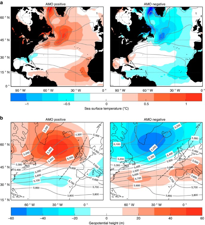
Figure 2: The spatial pattern of the AMO index and its relationship with the atmospheric flow in January. Composite maps of (a) sea surface temperature (SST) field and (b) 500 hPa geopotential height field (Z500) for AMO anomalously positive years (left panel) and negative years (right panel). The January mean field is shown in contours, and its departure from the 72-year climatology is represented by colour shading. The thick grey contour line in a denotes 0 °C, whereas thin (dashed) lines denote positive (negative) SST every 5 °C. The black dashed lines in b are drawn through the local maxima of the geopotential height field at each latitude, which is the point where the wind changes direction from south–westerly to north–westerly.
The large-scale atmospheric flow varies with the AMO index (Fig. 2b). The difference in the 500-hPa geopotential height (Z500) field, which is analogous to streamlines, shows that the direction of winds arriving in western Europe changes between the two AMO phases: winds are more northerly during the anomalous AMO-positive years, whereas they are more zonal during the AMO-negative years (Fig. 2b). The more tightly spaced isohypses during the AMO-negative years indicate a swifter flow relative to the AMO-positive years. Accordingly, the AMO-negative years see an elongated and more zonal January storm track (Supplementary Fig. 1), which is consistent with results from a free-running climate model7. Composite Z500 maps constructed with more complete sampling of the longer decadal periods associated with the AMO show similar, albeit weaker, anomaly patterns (Supplementary Fig. 2a).
In winter in the North Atlantic, SST is almost always warmer than the surface air temperature (SAT), so the ocean loses heat rapidly to the atmosphere over the entirety of the basin (that is, positive fluxes in our convention; Fig. 3b and Supplementary Fig. 3b). The fluxes over the warm Gulf Stream and its North Atlantic Current extension are generally a factor of five higher than found elsewhere. However, a view of the fluxes weighted by the fraction of time the particles spend in each location on their journey to western Europe (Fig. 3c and Supplementary Fig. 3c) suggests a reduced role of these strong flux regions in establishing western European wintertime temperature.
The difference in the number density of the particle positions between the composite AMO periods (Fig. 3d) shows a significant distinction in the preferred pathways, with the statistical significance increasing when results are separated by particles launched from northern and southern sub-regions of western Europe (Supplementary Fig. 3d). In the AMO-positive years, particles spend more of their 10-day trajectory recirculating locally to the southwest of Iceland. During the AMO-negative years, the pathways are anomalously long, and a greater number of trajectories originate from North America and the Arctic, before transiting over the Labrador Sea and mid-latitude North Atlantic.
The strengthening and lengthening of the storm track in sync with anomalously cooler North Atlantic SSTs has important implications for future climate. Given that decadal variability in North Atlantic SSTs may be driven partly by fluctuations in the strength of the AMOC10,11,12, our result suggests the possibility of a stabilizing feedback for ocean circulation: Cooler SSTs associated with a sluggish AMOC is linked with an atmospheric adjustment that enhances turbulent heat fluxes over oceanic convective regions in winter. These larger fluxes could possibly reinvigorate convection, deep water formation and the AMOC. Moreover, the observed link of the atmospheric circulation with the cool SST anomalies of the late 1970s to early 1990s is much like the predicted change of the storm track in response to a decline of the AMOC under global warming36. A weakened AMOC has long been thought to cause anomalous cooling in western Europe via a decline in oceanic heat transport and associated atmospheric feedbacks21. However, the changes we describe here in atmospheric Lagrangian trajectories and the heat fluxes along them could provide a mechanism that reduces the magnitude of European wintertime cooling on decadal time scales, even as they might stabilize the oceanic circulation.
The answer is blowin’ in the wind. Bob Dylan


/cdn.vox-cdn.com/uploads/chorus_asset/file/7389769/fww-bc-carbon-tax-emissions.png)


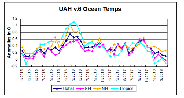
 The data is annual averages of absolute SSTs measured in the North Atlantic. The significance of the pulses for weather forecasting is discussed in
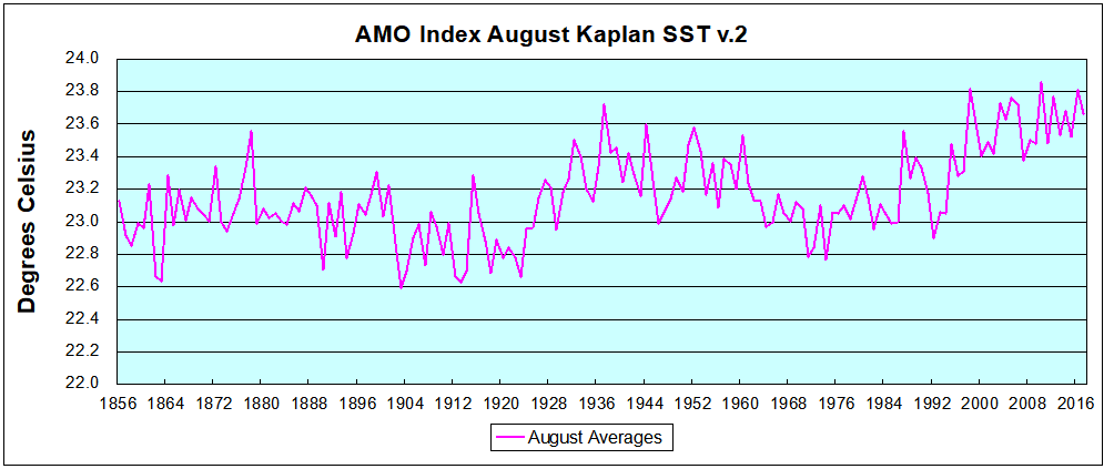


 Previous posts have discussed how the Judiciary seems unprepared for the mounting caseload of climate legal actions. Some background links are at the end, but this post is an update on two important court proceedings, thanks to Manhattan Contrarian Francis Menton. The essay is